|
|
| (4 intermediate revisions by the same user not shown) |
| Line 3,033: |
Line 3,033: |
| </tr> | | </tr> |
| </table> | | </table> |
| | |
| | This result should be compared with our [[SSC/Stability/BiPolytropes#Eigenfunction_Details|separate discussion of ''eigenfunction details'']]. |
|
| |
|
| ==Discretize for Numerical Integration== | | ==Discretize for Numerical Integration== |
| Line 4,047: |
Line 4,049: |
| </td></tr></table> | | </td></tr></table> |
|
| |
|
| ====Fourth Approximation==== | | =Part 2= |
| | |
| Let's assume that we know the four quantities, <math>x_{J-1}, x_J,(x_J)^' \equiv (dx/d\tilde{r})_J</math>, and <math>(x_{J-1})^' \equiv (dx/d\tilde{r})_{J-1}</math> and want to project forward to determine, <math>x_{J+1}</math>. We should assume that, locally, the displacement function <math>x</math> is cubic in <math>\tilde{r}</math>, that is,
| |
| | |
| <table border="0" align="center" cellpadding="5">
| |
| | |
| <tr>
| |
| <td align="right"><math>x</math></td>
| |
| <td align="center"><math>=</math></td>
| |
| <td align="left">
| |
| <math>
| |
| a + b\tilde{r} + c\tilde{r}^2 + e\tilde{r}^3
| |
| </math>
| |
| </td>
| |
| </tr>
| |
| | |
| <tr>
| |
| <td align="right"><math>\Rightarrow ~~~ \frac{dx}{d\tilde{r}}</math></td>
| |
| <td align="center"><math>=</math></td>
| |
| <td align="left">
| |
| <math>
| |
| b + 2c\tilde{r} + 3e\tilde{r}^2 \, ,
| |
| </math>
| |
| </td>
| |
| </tr>
| |
| </table>
| |
| where we have four unknowns, <math>a, b, c, e</math>. These can be determined by appropriately combining the four relations,
| |
| | |
| <table border="0" align="center" cellpadding="5">
| |
| | |
| <tr>
| |
| <td align="right"><math>(x_J)^'</math></td>
| |
| <td align="center"><math>=</math></td>
| |
| <td align="left">
| |
| <math>
| |
| b + 2c\tilde{r}_J + 3e\tilde{r}_J^2\, ,
| |
| </math>
| |
| </td>
| |
| </tr>
| |
| | |
| <tr>
| |
| <td align="right"><math>(x_{J-1})^'</math></td>
| |
| <td align="center"><math>=</math></td>
| |
| <td align="left">
| |
| <math>
| |
| b + 2c(\tilde{r}_J - \Delta\tilde{r}) + 3e(\tilde{r}_J - \Delta\tilde{r})^2\, ,
| |
| </math>
| |
| </td>
| |
| </tr>
| |
| | |
| <tr>
| |
| <td align="right"><math>x_J</math></td>
| |
| <td align="center"><math>=</math></td>
| |
| <td align="left">
| |
| <math>
| |
| a + b\tilde{r}_J + c\tilde{r}_J^2 + e\tilde{r}_J^3\, ,
| |
| </math>
| |
| </td>
| |
| </tr>
| |
| | |
| <tr>
| |
| <td align="right"><math>x_{J-1}</math></td>
| |
| <td align="center"><math>=</math></td>
| |
| <td align="left">
| |
| <math>
| |
| a + b(\tilde{r}_{J}-\Delta\tilde{r}) + c(\tilde{r}_{J}-\Delta\tilde{r})^2 + e(\tilde{r}_J - \Delta\tilde{r})^3 \, ,
| |
| </math>
| |
| </td>
| |
| </tr>
| |
| </table>
| |
| The difference between the first two expressions gives,
| |
| | |
| <table border="0" align="center" cellpadding="5">
| |
| | |
| <tr>
| |
| <td align="right"><math>(x_J)^' - (x_{J-1})^'</math></td>
| |
| <td align="center"><math>=</math></td>
| |
| <td align="left">
| |
| <math>
| |
| [2c\tilde{r}_J + 3e\tilde{r}_J^2]
| |
| -
| |
| [2c(\tilde{r}_J - \Delta\tilde{r}) + 3e(\tilde{r}_J - \Delta\tilde{r})^2]
| |
| </math>
| |
| </td>
| |
| </tr>
| |
| | |
| <tr>
| |
| <td align="right"> </td>
| |
| <td align="center"><math>=</math></td>
| |
| <td align="left">
| |
| <math>2c\tilde{r}_J + 3e\tilde{r}_J^2-[2c\tilde{r}_J - 2c\Delta\tilde{r} + 3e(\tilde{r}_J^2 - 2\tilde{r}_J\Delta\tilde{r} + \Delta\tilde{r}^2)]
| |
| </math>
| |
| </td>
| |
| </tr>
| |
| | |
| <tr>
| |
| <td align="right"> </td>
| |
| <td align="center"><math>=</math></td>
| |
| <td align="left">
| |
| <math>
| |
| 2c\Delta\tilde{r} + 6e\tilde{r}_J\Delta\tilde{r} - 3e\Delta\tilde{r}^2
| |
| </math>
| |
| </td>
| |
| </tr>
| |
| | |
| <tr>
| |
| <td align="right"><math>\Rightarrow ~~~ 2c\Delta\tilde{r}</math>
| |
| </td>
| |
| <td align="center"><math>=</math></td>
| |
| <td align="left">
| |
| <math>
| |
| \biggl[ (x_J)^' - (x_{J-1})^'\biggr] + 3e\Delta\tilde{r}^2 - 6e\tilde{r}_J\Delta\tilde{r}
| |
| </math>
| |
| </td>
| |
| </tr>
| |
| | |
| <tr>
| |
| <td align="right"><math>\Rightarrow ~~~ c</math>
| |
| </td>
| |
| <td align="center"><math>=</math></td>
| |
| <td align="left">
| |
| <math>
| |
| \biggl[ \frac{(x_J)^' - (x_{J-1})^'}{2\Delta\tilde{r}}\biggr] + 3e\biggl[\frac{\Delta\tilde{r}}{2}- \tilde{r}_J \biggr] \, .
| |
| </math>
| |
| </td>
| |
| </tr>
| |
| </table>
| |
| | |
| And the difference between the last two expressions gives,
| |
| | |
| <table border="0" align="center" cellpadding="5">
| |
| | |
| <tr>
| |
| <td align="right"><math>x_J - x_{J-1}</math></td>
| |
| <td align="center"><math>=</math></td>
| |
| <td align="left">
| |
| <math>
| |
| \biggl[ b\tilde{r}_J + c\tilde{r}_J^2 + e\tilde{r}_J^3\biggr]
| |
| -
| |
| \biggl[ b(\tilde{r}_{J}-\Delta\tilde{r}) + c(\tilde{r}_{J}-\Delta\tilde{r})^2 + e(\tilde{r}_J - \Delta\tilde{r})^3\biggr]
| |
| </math>
| |
| </td>
| |
| </tr>
| |
| | |
| <tr>
| |
| <td align="right"> </td>
| |
| <td align="center"><math>=</math></td>
| |
| <td align="left">
| |
| <math>
| |
| b\Delta\tilde{r}
| |
| +
| |
| c(2\tilde{r}_J \Delta\tilde{r} - \Delta\tilde{r}^2)
| |
| + e\tilde{r}_J^3 - e(\tilde{r}_J - \Delta\tilde{r})(\tilde{r}_J^2 - 2\tilde{r}_J\Delta\tilde{r} + \Delta\tilde{r}^2)
| |
| </math>
| |
| </td>
| |
| </tr>
| |
| | |
| <tr>
| |
| <td align="right"> </td>
| |
| <td align="center"><math>=</math></td>
| |
| <td align="left">
| |
| <math>
| |
| b\Delta\tilde{r}
| |
| +
| |
| c(2\tilde{r}_J \Delta\tilde{r} - \Delta\tilde{r}^2)
| |
| + e\tilde{r}_J^3 - e\biggl[
| |
| (\tilde{r}_J )(\tilde{r}_J^2 - 2\tilde{r}_J\Delta\tilde{r} + \Delta\tilde{r}^2)
| |
| -
| |
| (\Delta\tilde{r})(\tilde{r}_J^2 - 2\tilde{r}_J\Delta\tilde{r} + \Delta\tilde{r}^2)
| |
| \biggr]
| |
| </math>
| |
| </td>
| |
| </tr>
| |
| | |
| <tr>
| |
| <td align="right"> </td>
| |
| <td align="center"><math>=</math></td>
| |
| <td align="left">
| |
| <math>
| |
| b\Delta\tilde{r}
| |
| +
| |
| c(2\tilde{r}_J \Delta\tilde{r} - \Delta\tilde{r}^2)
| |
| - e\biggl[
| |
| - 3\tilde{r}_J^2\Delta\tilde{r} + 3\tilde{r}_J\Delta\tilde{r}^2
| |
| -\Delta\tilde{r}^3
| |
| \biggr]
| |
| </math>
| |
| </td>
| |
| </tr>
| |
| | |
| <tr>
| |
| <td align="right"> </td>
| |
| <td align="center"><math>=</math></td>
| |
| <td align="left">
| |
| <math>
| |
| b\Delta\tilde{r}
| |
| +
| |
| c(2\tilde{r}_J \Delta\tilde{r} - \Delta\tilde{r}^2)
| |
| + e\biggl[
| |
| 3\tilde{r}_J^2\Delta\tilde{r} - 3\tilde{r}_J\Delta\tilde{r}^2
| |
| + \Delta\tilde{r}^3
| |
| \biggr]
| |
| </math>
| |
| </td>
| |
| </tr>
| |
| | |
| <tr>
| |
| <td align="right"><math>\Rightarrow ~~~ b\Delta\tilde{r}</math></td>
| |
| <td align="center"><math>=</math></td>
| |
| <td align="left">
| |
| <math>
| |
| \biggl[x_J - x_{J-1}\biggr]
| |
| +
| |
| 2c\Delta\tilde{r}\biggl[ \frac{\Delta\tilde{r}}{2} - \tilde{r}_J\biggr]
| |
| - e\biggl[
| |
| 3\tilde{r}_J^2\Delta\tilde{r} - 3\tilde{r}_J\Delta\tilde{r}^2
| |
| + \Delta\tilde{r}^3
| |
| \biggr]
| |
| </math>
| |
| </td>
| |
| </tr>
| |
| | |
| <tr>
| |
| <td align="right"> </td>
| |
| <td align="center"><math>=</math></td>
| |
| <td align="left">
| |
| <math>
| |
| \biggl[x_J - x_{J-1}\biggr]
| |
| +
| |
| \biggl\{
| |
| \biggl[ (x_J)^' - (x_{J-1})^'\biggr] + 3e\Delta\tilde{r}\biggl[ \Delta\tilde{r} - 2\tilde{r}_J\biggr]
| |
| \biggr\}
| |
| \biggl[ \frac{\Delta\tilde{r}}{2} - \tilde{r}_J\biggr]
| |
| - 3e\Delta\tilde{r} \biggl[
| |
| \tilde{r}_J^2 - \tilde{r}_J\Delta\tilde{r}
| |
| + \frac{\Delta\tilde{r}^2}{3}
| |
| \biggr]
| |
| </math>
| |
| </td>
| |
| </tr>
| |
| | |
| <tr>
| |
| <td align="right"> </td>
| |
| <td align="center"><math>=</math></td>
| |
| <td align="left">
| |
| <math>
| |
| \biggl[x_J - x_{J-1}\biggr]
| |
| +
| |
| \biggl[ (x_J)^' - (x_{J-1})^'\biggr]\biggl[ \frac{\Delta\tilde{r}}{2} - \tilde{r}_J\biggr]
| |
| | |
| + 3e\Delta\tilde{r}
| |
| \biggl[ \frac{\Delta\tilde{r}^2}{2} - \tilde{r}_J \Delta\tilde{r}\biggr]
| |
| | |
| - 3e\Delta\tilde{r}
| |
| \biggl[ \tilde{r}_J\Delta\tilde{r} - 2\tilde{r}_J^2\biggr]
| |
| | |
| - 3e\Delta\tilde{r} \biggl[
| |
| \tilde{r}_J^2 - \tilde{r}_J\Delta\tilde{r}
| |
| + \frac{\Delta\tilde{r}^2}{3}
| |
| \biggr]
| |
| </math>
| |
| </td>
| |
| </tr>
| |
| | |
| <tr>
| |
| <td align="right"> </td>
| |
| <td align="center"><math>=</math></td>
| |
| <td align="left">
| |
| <math>
| |
| \biggl[x_J - x_{J-1}\biggr]
| |
| +
| |
| \biggl[ (x_J)^' - (x_{J-1})^'\biggr]\biggl[ \frac{\Delta\tilde{r}}{2} - \tilde{r}_J\biggr]
| |
| | |
| - 3e\Delta\tilde{r}\biggl\{
| |
| \biggl[ \tilde{r}_J \Delta\tilde{r} - \frac{\Delta\tilde{r}^2}{2} \biggr]
| |
| | |
| +
| |
| \biggl[ \tilde{r}_J\Delta\tilde{r} - 2\tilde{r}_J^2\biggr]
| |
| | |
| + \biggl[
| |
| \tilde{r}_J^2 - \tilde{r}_J\Delta\tilde{r}
| |
| + \frac{\Delta\tilde{r}^2}{3}
| |
| \biggr]
| |
| \biggr\}
| |
| </math>
| |
| </td>
| |
| </tr>
| |
| | |
| <tr>
| |
| <td align="right"> </td>
| |
| <td align="center"><math>=</math></td>
| |
| <td align="left">
| |
| <math>
| |
| \biggl[x_J - x_{J-1}\biggr]
| |
| +
| |
| \biggl[ (x_J)^' - (x_{J-1})^'\biggr]\biggl[ \frac{\Delta\tilde{r}}{2} - \tilde{r}_J\biggr]
| |
| | |
| + e\Delta\tilde{r}\biggl[
| |
| 3\tilde{r}_J^2
| |
| - 3\tilde{r}_J \Delta\tilde{r}
| |
| + \frac{\Delta\tilde{r}^2}{2}
| |
| \biggr]
| |
| \, .
| |
| </math>
| |
| </td>
| |
| </tr>
| |
| </table>
| |
| | |
| <table border="1" width="80%" cellpadding="8" align="center"><tr><td align="left">
| |
| <div align="center"><b>Summary #1:</b></div>
| |
| In terms of the coefficient, <math>e</math> …
| |
| | |
| <table border="0" align="center" cellpadding="5">
| |
| | |
| <tr>
| |
| <td align="right"><math>b \Delta\tilde{r}</math></td>
| |
| <td align="center"><math>=</math></td>
| |
| <td align="left">
| |
| <math>
| |
| \biggl[x_J - x_{J-1}\biggr]
| |
| +
| |
| \biggl[ (x_J)^' - (x_{J-1})^'\biggr]\biggl[ \frac{\Delta\tilde{r}}{2} - \tilde{r}_J\biggr]
| |
| | |
| + e\Delta\tilde{r}\biggl[
| |
| 3\tilde{r}_J^2
| |
| - 3\tilde{r}_J \Delta\tilde{r}
| |
| + \frac{\Delta\tilde{r}^2}{2}
| |
| \biggr]
| |
| \, ,
| |
| </math>
| |
| </td>
| |
| </tr>
| |
| | |
| <tr>
| |
| <td align="right"><math>2c\Delta\tilde{r}</math>
| |
| </td>
| |
| <td align="center"><math>=</math></td>
| |
| <td align="left">
| |
| <math>
| |
| \biggl[ (x_J)^' - (x_{J-1})^'\biggr] + e\Delta\tilde{r}\biggl[ 3\Delta\tilde{r} - 6\tilde{r}_J \biggr]
| |
| \, .
| |
| </math>
| |
| </td>
| |
| </tr>
| |
| </table>
| |
| | |
| </td></tr></table>
| |
| Hence, from the first of the four relations, we find that,
| |
| | |
| <table border="0" align="center" cellpadding="5">
| |
| | |
| <tr>
| |
| <td align="right"><math>(x_J)^'\Delta\tilde{r} - 3e\tilde{r}_J^2\Delta\tilde{r}</math></td>
| |
| <td align="center"><math>=</math></td>
| |
| <td align="left">
| |
| <math>
| |
| (b\Delta\tilde{r}) + (2c\Delta\tilde{r}) \tilde{r}_J
| |
| </math>
| |
| </td>
| |
| </tr>
| |
| | |
| <tr>
| |
| <td align="right"> </td>
| |
| <td align="center"><math>=</math></td>
| |
| <td align="left">
| |
| <math>
| |
| \biggl[x_J - x_{J-1}\biggr]
| |
| +
| |
| \biggl[ (x_J)^' - (x_{J-1})^'\biggr]\biggl[ \frac{\Delta\tilde{r}}{2} - \tilde{r}_J\biggr]
| |
| | |
| + e\Delta\tilde{r}\biggl[
| |
| 3\tilde{r}_J^2
| |
| - 3\tilde{r}_J \Delta\tilde{r}
| |
| + \frac{\Delta\tilde{r}^2}{2}
| |
| \biggr]
| |
| +
| |
| \biggl\{
| |
| \biggl[ (x_J)^' - (x_{J-1})^'\biggr] + e\Delta\tilde{r}\biggl[ 3\Delta\tilde{r} - 6\tilde{r}_J \biggr]
| |
| \biggr\} \tilde{r}_J
| |
| </math>
| |
| </td>
| |
| </tr>
| |
| | |
| <tr>
| |
| <td align="right"> </td>
| |
| <td align="center"><math>=</math></td>
| |
| <td align="left">
| |
| <math>
| |
| \biggl[x_J - x_{J-1}\biggr]
| |
| +
| |
| \biggl[ (x_J)^' - (x_{J-1})^'\biggr]\biggl[ \frac{\Delta\tilde{r}}{2} \biggr]
| |
| | |
| + e\Delta\tilde{r}\biggl[
| |
| 3\tilde{r}_J^2
| |
| - 3\tilde{r}_J \Delta\tilde{r}
| |
| + \frac{\Delta\tilde{r}^2}{2}
| |
| \biggr]
| |
| +
| |
| e\Delta\tilde{r}\biggl[ 3\tilde{r}_J\Delta\tilde{r} - 6\tilde{r}_J^2 \biggr]
| |
| </math>
| |
| </td>
| |
| </tr>
| |
| | |
| <tr>
| |
| <td align="right"> </td>
| |
| <td align="center"><math>=</math></td>
| |
| <td align="left">
| |
| <math>
| |
| \biggl[x_J - x_{J-1}\biggr]
| |
| +
| |
| \biggl[ (x_J)^' - (x_{J-1})^'\biggr]\biggl[ \frac{\Delta\tilde{r}}{2} \biggr]
| |
| | |
| + e\Delta\tilde{r}\biggl[
| |
| -3\tilde{r}_J^2
| |
| + \frac{\Delta\tilde{r}^2}{2}
| |
| \biggr]
| |
| </math>
| |
| </td>
| |
| </tr>
| |
| | |
| <tr>
| |
| <td align="right"><math>\Rightarrow ~~~ (x_J)^'\Delta\tilde{r} </math></td>
| |
| <td align="center"><math>=</math></td>
| |
| <td align="left">
| |
| <math>
| |
| \biggl[x_J - x_{J-1}\biggr]
| |
| +
| |
| \biggl[ (x_J)^' - (x_{J-1})^'\biggr]\biggl[ \frac{\Delta\tilde{r}}{2} \biggr]
| |
| | |
| + e\biggl[\frac{\Delta\tilde{r}^3}{2} \biggr]
| |
| </math>
| |
| </td>
| |
| </tr>
| |
| | |
| <tr>
| |
| <td align="right"><math>\Rightarrow ~~~ e\biggl[\frac{\Delta\tilde{r}^3}{2} \biggr] </math></td>
| |
| <td align="center"><math>=</math></td>
| |
| <td align="left">
| |
| <math>
| |
| - \biggl[x_J - x_{J-1}\biggr]
| |
| -
| |
| \biggl[ (x_J)^' - (x_{J-1})^'\biggr]\biggl[ \frac{\Delta\tilde{r}}{2} \biggr]
| |
| | |
| + (x_J)^'\Delta\tilde{r}
| |
| </math>
| |
| </td>
| |
| </tr>
| |
| | |
| <tr>
| |
| <td align="right"> </td>
| |
| <td align="center"><math>=</math></td>
| |
| <td align="left">
| |
| <math>
| |
| \biggl[x_{J-1} - x_J \biggr]
| |
| +
| |
| \biggl[(x_{J-1})^'+ (x_J)^' \biggr] \frac{\Delta\tilde{r}}{2}
| |
| </math>
| |
| </td>
| |
| </tr>
| |
| | |
| <tr>
| |
| <td align="right"><math>\Rightarrow ~~~ e \Delta\tilde{r}^3 </math></td>
| |
| <td align="center"><math>=</math></td>
| |
| <td align="left">
| |
| <math>
| |
| 2\biggl[x_{J-1} - x_J \biggr]
| |
| +
| |
| \biggl[(x_{J-1})^'+ (x_J)^' \biggr] \Delta\tilde{r} \, .
| |
| </math>
| |
| </td>
| |
| </tr>
| |
| </table>
| |
| | |
| Finally, from the third of the four relations, we can evaluate the coefficient, <math>a</math>; specifically,
| |
| | |
| <table border="0" align="center" cellpadding="5">
| |
| | |
| <tr>
| |
| <td align="right"><math>x_J - a - e\tilde{r}_J^3</math></td>
| |
| <td align="center"><math>=</math></td>
| |
| <td align="left">
| |
| <math>
| |
| b\tilde{r}_J + c\tilde{r}_J^2
| |
| </math>
| |
| </td>
| |
| </tr>
| |
| | |
| <tr>
| |
| <td align="right"> </td>
| |
| <td align="center"><math>=</math></td>
| |
| <td align="left">
| |
| <math>
| |
| \frac{\tilde{r}_J}{\Delta\tilde{r}} \biggl\{ b\Delta\tilde{r} \biggr\}
| |
| +
| |
| \frac{\tilde{r}_J^2}{2\Delta\tilde{r}} \biggl\{2c\Delta\tilde{r}\biggr\}
| |
| </math>
| |
| </td>
| |
| </tr>
| |
| | |
| <tr>
| |
| <td align="right"> </td>
| |
| <td align="center"><math>=</math></td>
| |
| <td align="left">
| |
| <math>
| |
| \frac{\tilde{r}_J}{\Delta\tilde{r}} \biggl\{
| |
| \biggl[x_J - x_{J-1}\biggr]
| |
| +
| |
| \biggl[ (x_J)^' - (x_{J-1})^'\biggr]\biggl[ \frac{\Delta\tilde{r}}{2} - \tilde{r}_J\biggr]
| |
| | |
| + e\Delta\tilde{r}\biggl[
| |
| 3\tilde{r}_J^2
| |
| - 3\tilde{r}_J \Delta\tilde{r}
| |
| + \frac{\Delta\tilde{r}^2}{2}
| |
| \biggr]
| |
| \biggr\}
| |
| +
| |
| \frac{\tilde{r}_J^2}{2\Delta\tilde{r}} \biggl\{
| |
| \biggl[ (x_J)^' - (x_{J-1})^'\biggr] + e\Delta\tilde{r}\biggl[ 3\Delta\tilde{r} - 6\tilde{r}_J \biggr]
| |
| \biggr\}
| |
| </math>
| |
| </td>
| |
| </tr>
| |
| | |
| <tr>
| |
| <td align="right"> </td>
| |
| <td align="center"><math>=</math></td>
| |
| <td align="left">
| |
| <math>
| |
| \biggl\{
| |
| \frac{\tilde{r}_J}{\Delta\tilde{r}} \biggl[x_J - x_{J-1}\biggr]
| |
| +
| |
| \frac{\tilde{r}_J}{\Delta\tilde{r}} \biggl[ (x_J)^' - (x_{J-1})^'\biggr]\biggl[ \frac{\Delta\tilde{r}}{2} - \tilde{r}_J\biggr]
| |
| | |
| + e\tilde{r}_J \biggl[
| |
| 3\tilde{r}_J^2
| |
| - 3\tilde{r}_J \Delta\tilde{r}
| |
| + \frac{\Delta\tilde{r}^2}{2}
| |
| \biggr]
| |
| \biggr\}
| |
| +
| |
| \biggl\{
| |
| \frac{\tilde{r}_J^2}{2\Delta\tilde{r}} \biggl[ (x_J)^' - (x_{J-1})^'\biggr]
| |
| + \frac{e\tilde{r}_J^2}{2} \biggl[ 3\Delta\tilde{r} - 6\tilde{r}_J \biggr]
| |
| \biggr\}
| |
| </math>
| |
| </td>
| |
| </tr>
| |
| | |
| <tr>
| |
| <td align="right"> </td>
| |
| <td align="center"><math>=</math></td>
| |
| <td align="left">
| |
| <math>
| |
| \frac{\tilde{r}_J}{\Delta\tilde{r}} \biggl[x_J - x_{J-1}\biggr]
| |
| +
| |
| \biggl[ (x_J)^' - (x_{J-1})^'\biggr]\biggl[ \frac{\tilde{r}_J}{2} - \frac{\tilde{r}_J^2}{2\Delta\tilde{r}}\biggr]
| |
| | |
| + e \biggl[
| |
| 3\tilde{r}_J^3
| |
| - 3\tilde{r}_J^2 \Delta\tilde{r}
| |
| + \frac{\tilde{r}_J\Delta\tilde{r}^2}{2}
| |
| \biggr]
| |
| +
| |
| e\biggl[ \frac{3\tilde{r}_J^2 \Delta\tilde{r}}{2} - 3\tilde{r}_J^3 \biggr]
| |
| </math>
| |
| </td>
| |
| </tr>
| |
| | |
| <tr>
| |
| <td align="right"> </td>
| |
| <td align="center"><math>=</math></td>
| |
| <td align="left">
| |
| <math>
| |
| \frac{\tilde{r}_J}{\Delta\tilde{r}} \biggl[x_J - x_{J-1}\biggr]
| |
| +
| |
| \frac{1}{2\Delta\tilde{r}}\biggl[ (x_J)^' - (x_{J-1})^'\biggr]\biggl[ \tilde{r}_J \Delta\tilde{r} - \tilde{r}_J^2\biggr]
| |
| | |
| + \frac{e\Delta\tilde{r}}{2} \biggl[
| |
| \tilde{r}_J\Delta\tilde{r}
| |
| -3\tilde{r}_J^2 \biggr] \, .
| |
| </math>
| |
| </td>
| |
| </tr>
| |
| </table>
| |
| That is,
| |
| | |
| <table border="0" align="center" cellpadding="5">
| |
| | |
| <tr>
| |
| <td align="right"><math>a </math></td>
| |
| <td align="center"><math>=</math></td>
| |
| <td align="left">
| |
| <math>
| |
| x_J -\frac{\tilde{r}_J}{\Delta\tilde{r}} \biggl[x_J - x_{J-1}\biggr]
| |
| -
| |
| \frac{1}{2\Delta\tilde{r}}\biggl[ (x_J)^' - (x_{J-1})^'\biggr]\biggl[ \tilde{r}_J \Delta\tilde{r} - \tilde{r}_J^2\biggr]
| |
| | |
| - e\biggl\{
| |
| \frac{\Delta\tilde{r}}{2} \biggl[
| |
| \tilde{r}_J\Delta\tilde{r}
| |
| -3\tilde{r}_J^2 \biggr]
| |
| + \tilde{r}_J^3
| |
| \biggr\}
| |
| </math>
| |
| </td>
| |
| </tr>
| |
| | |
| <tr>
| |
| <td align="right"> </td>
| |
| <td align="center"><math>=</math></td>
| |
| <td align="left">
| |
| <math>
| |
| x_J -\frac{\tilde{r}_J}{\Delta\tilde{r}} \biggl[x_J - x_{J-1}\biggr]
| |
| -
| |
| \frac{1}{2\Delta\tilde{r}}\biggl[ (x_J)^' - (x_{J-1})^'\biggr]\biggl[ \tilde{r}_J \Delta\tilde{r} - \tilde{r}_J^2\biggr]
| |
| | |
| - e\Delta\tilde{r}^3\biggl\{
| |
| \frac{1}{2\Delta\tilde{r}^2} \biggl[
| |
| \tilde{r}_J\Delta\tilde{r}
| |
| -3\tilde{r}_J^2 \biggr]
| |
| + \biggl(\frac{\tilde{r}_J}{\Delta\tilde{r}}\biggr)^3
| |
| \biggr\}
| |
| </math>
| |
| </td>
| |
| </tr>
| |
| </table>
| |
| | |
| <table border="1" width="80%" cellpadding="8" align="center"><tr><td align="left">
| |
| <div align="center"><b>Summary #2:</b></div>
| |
| In terms of the coefficient, <math>e</math> …
| |
| | |
| <table border="0" align="center" cellpadding="5">
| |
| | |
| <tr>
| |
| <td align="right"><math>a</math></td>
| |
| <td align="center"><math>=</math></td>
| |
| <td align="left">
| |
| <math>
| |
| x_J -\frac{\tilde{r}_J}{\Delta\tilde{r}} \biggl[x_J - x_{J-1}\biggr]
| |
| -
| |
| \frac{1}{2\Delta\tilde{r}}\biggl[ (x_J)^' - (x_{J-1})^'\biggr]\biggl[ \tilde{r}_J \Delta\tilde{r} - \tilde{r}_J^2\biggr]
| |
| | |
| - e\Delta\tilde{r}^3\biggl\{
| |
| \frac{1}{2\Delta\tilde{r}^2} \biggl[
| |
| \tilde{r}_J\Delta\tilde{r}
| |
| -3\tilde{r}_J^2 \biggr]
| |
| + \biggl(\frac{\tilde{r}_J}{\Delta\tilde{r}}\biggr)^3
| |
| \biggr\} \, ,
| |
| </math>
| |
| </td>
| |
| </tr>
| |
| | |
| <tr>
| |
| <td align="right"><math>b \Delta\tilde{r}</math></td>
| |
| <td align="center"><math>=</math></td>
| |
| <td align="left">
| |
| <math>
| |
| \biggl[x_J - x_{J-1}\biggr]
| |
| +
| |
| \biggl[ (x_J)^' - (x_{J-1})^'\biggr]\biggl[ \frac{\Delta\tilde{r}}{2} - \tilde{r}_J\biggr]
| |
| | |
| + e\Delta\tilde{r}^3\biggl[
| |
| \frac{3\tilde{r}_J^2}{\Delta\tilde{r}^2}
| |
| - \frac{3\tilde{r}_J}{ \Delta\tilde{r} }
| |
| + \frac{1}{2}
| |
| \biggr]
| |
| \, ,
| |
| </math>
| |
| </td>
| |
| </tr>
| |
| | |
| <tr>
| |
| <td align="right"><math>c\Delta\tilde{r}^2</math>
| |
| </td>
| |
| <td align="center"><math>=</math></td>
| |
| <td align="left">
| |
| <math>
| |
| \biggl[ (x_J)^' - (x_{J-1})^'\biggr]\frac{\Delta\tilde{r}}{2}
| |
| +
| |
| e\Delta\tilde{r}^3\biggl[ \frac{3}{2} - \frac{3\tilde{r}_J}{\Delta\tilde{r}} \biggr]
| |
| \, ,
| |
| </math>
| |
| </td>
| |
| </tr>
| |
| | |
| <tr>
| |
| <td align="right"><math>e \Delta\tilde{r}^3 </math></td>
| |
| <td align="center"><math>=</math></td>
| |
| <td align="left">
| |
| <math>
| |
| 2\biggl[x_{J-1} - x_J \biggr]
| |
| +
| |
| \biggl[(x_{J-1})^'+ (x_J)^' \biggr] \Delta\tilde{r} \, .
| |
| </math>
| |
| </td>
| |
| </tr>
| |
| </table>
| |
| | |
| </td></tr></table>
| |
| | |
| <table border=1 align="center" cellpadding="10" width="80%"><tr><td bgcolor="pink" align="left">
| |
| This is test ...
| |
| <table border="1" align="center" cellpadding="5">
| |
| | |
| <tr>
| |
| <td align="center" bgcolor="white"><math>\tilde{r}_J = \tilde{r}_i + \Delta\tilde{r}</math></td>
| |
| <td align="center" bgcolor="white"><math>\Delta\tilde{r}</math></td>
| |
| <td align="center" bgcolor="white"><math>x_J</math></td>
| |
| <td align="center" bgcolor="white"><math>x_{J-1}</math></td>
| |
| <td align="center" bgcolor="white"><math>(x_J)^'</math></td>
| |
| <td align="center" bgcolor="white"><math>(x_{J-1})^'</math></td>
| |
| </tr>
| |
| | |
| <tr>
| |
| <td align="center" bgcolor="white">0.01740039</td>
| |
| <td align="center" bgcolor="white">0.001936393</td>
| |
| <td align="center" bgcolor="white">-4.695376</td>
| |
| <td align="center" bgcolor="white">-4.547832</td>
| |
| <td align="center" bgcolor="white">-116.0119</td>
| |
| <td align="center" bgcolor="white">-76.19513</td>
| |
| </tr>
| |
| </table>
| |
| </td></tr>
| |
| <tr><td bgcolor="white" align="left">
| |
| | |
| <table border="0" align="center" cellpadding="5">
| |
| | |
| <tr>
| |
| <td align="right"><math>a</math></td>
| |
| <td align="center"><math>=</math></td>
| |
| <td align="left">
| |
| <math>
| |
| -3.36955 -2.76645 - e\Delta\tilde{r}^3(608.9698) = -232.7874
| |
| \, ,
| |
| </math>
| |
| </td>
| |
| </tr>
| |
| | |
| <tr>
| |
| <td align="right"><math>b \Delta\tilde{r}</math></td>
| |
| <td align="center"><math>=</math></td>
| |
| <td align="left">
| |
| <math>
| |
| 0.5067329 + e\Delta\tilde{r}^3 (215.7856) = +80.819698
| |
| \, ,
| |
| </math>
| |
| </td>
| |
| </tr>
| |
| | |
| <tr>
| |
| <td align="right"><math>c\Delta\tilde{r}^2</math>
| |
| </td>
| |
| <td align="center"><math>=</math></td>
| |
| <td align="left">
| |
| <math>
| |
| -0.0385505 + e\Delta\tilde{r}^3 ( -25.45794 ) = -9.51370
| |
| \, ,
| |
| </math>
| |
| </td>
| |
| </tr>
| |
| | |
| <tr>
| |
| <td align="right"><math>e \Delta\tilde{r}^3 </math></td>
| |
| <td align="center"><math>=</math></td>
| |
| <td align="left">
| |
| <math>
| |
| 0.3721883
| |
| \, .
| |
| </math>
| |
| </td>
| |
| </tr>
| |
| </table>
| |
| | |
| Hence,
| |
| | |
| <table border="0" align="center" cellpadding="5">
| |
| | |
| <tr>
| |
| <td align="right"><math>x_J </math></td>
| |
| <td align="center"><math>=</math></td>
| |
| <td align="left">
| |
| <math>
| |
| a
| |
| + b\Delta\tilde{r} \biggl( \frac{\tilde{r}_J}{\Delta\tilde{r}} \biggr)
| |
| + c\Delta\tilde{r}^2 \biggl( \frac{\tilde{r}_J}{\Delta\tilde{r}} \biggr)^2
| |
| + e\Delta\tilde{r}^3 \biggl( \frac{\tilde{r}_J}{\Delta\tilde{r}} \biggr)^3
| |
| </math>
| |
| </td>
| |
| </tr>
| |
| | |
| <tr>
| |
| <td align="right"> </td>
| |
| <td align="center"><math>=</math></td>
| |
| <td align="left">
| |
| <math>
| |
| -232.7874 +726.2442 -768.2108 +270.0593 = -4.68369 \, .
| |
| </math>
| |
| </td>
| |
| </tr>
| |
| </table>
| |
| Higher precision value (from Excel) is <math>x_J = -4.695376 \, ,</math> which precisely matches the input value.
| |
| </td></tr></table>
| |
| | |
| As a result,
| |
| | |
| <table border="0" align="center" cellpadding="5">
| |
| | |
| <tr>
| |
| <td align="right"><math>x_{J+1}</math></td>
| |
| <td align="center"><math>=</math></td>
| |
| <td align="left">
| |
| <math>
| |
| \biggl\{
| |
| a
| |
| \biggr\}
| |
| + (\tilde{r}_J +\Delta\tilde{r}) \biggl\{
| |
| b
| |
| \biggr\}
| |
| + (\tilde{r}_J+\Delta\tilde{r})^2 \biggl\{
| |
| c
| |
| \biggr\}
| |
| + (\tilde{r}_J+\Delta\tilde{r})^3 \biggl\{
| |
| e
| |
| \biggr\}
| |
| </math>
| |
| </td>
| |
| </tr>
| |
| | |
| <tr>
| |
| <td align="right"> </td>
| |
| <td align="center"><math>=</math></td>
| |
| <td align="left">
| |
| <math>
| |
| \biggl\{
| |
| a
| |
| \biggr\}
| |
| + \biggl( \frac{\tilde{r}_J}{\Delta\tilde{r}} + 1\biggr) \biggl\{
| |
| b\Delta\tilde{r}
| |
| \biggr\}
| |
| + \biggl( \frac{\tilde{r}_J}{\Delta\tilde{r}} + 1\biggr)^2 \biggl\{
| |
| c\Delta\tilde{r}^2
| |
| \biggr\}
| |
| + \biggl( \frac{\tilde{r}_J}{\Delta\tilde{r}} + 1\biggr)^3 \biggl\{
| |
| e\Delta\tilde{r}^3
| |
| \biggr\}
| |
| </math>
| |
| </td>
| |
| </tr>
| |
| | |
| <tr>
| |
| <td align="right"> </td>
| |
| <td align="center"><math>=</math></td>
| |
| <td align="left">
| |
| <math>
| |
| x_J -\frac{\tilde{r}_J}{\Delta\tilde{r}} \biggl[x_J - x_{J-1}\biggr]
| |
| -
| |
| \frac{1}{2\Delta\tilde{r}}\biggl[ (x_J)^' - (x_{J-1})^'\biggr]\biggl[ \tilde{r}_J \Delta\tilde{r} - \tilde{r}_J^2\biggr]
| |
| | |
| - e\Delta\tilde{r}^3\biggl\{
| |
| \frac{1}{2\Delta\tilde{r}^2} \biggl[
| |
| \tilde{r}_J\Delta\tilde{r}
| |
| -3\tilde{r}_J^2 \biggr]
| |
| + \biggl(\frac{\tilde{r}_J}{\Delta\tilde{r}}\biggr)^3
| |
| \biggr\}
| |
| </math>
| |
| </td>
| |
| </tr>
| |
| | |
| <tr>
| |
| <td align="right"> </td>
| |
| <td align="center"> </td>
| |
| <td align="left">
| |
| <math>
| |
| + \biggl( \frac{\tilde{r}_J}{\Delta\tilde{r}} + 1\biggr) \biggl\{
| |
| \biggl[x_J - x_{J-1}\biggr]
| |
| +
| |
| \biggl[ (x_J)^' - (x_{J-1})^'\biggr]\biggl[ \frac{\Delta\tilde{r}}{2} - \tilde{r}_J\biggr]
| |
| | |
| + e\Delta\tilde{r}^3\biggl[
| |
| \frac{3\tilde{r}_J^2}{\Delta\tilde{r}^2}
| |
| - \frac{3\tilde{r}_J}{ \Delta\tilde{r} }
| |
| + \frac{1}{2}
| |
| \biggr]
| |
| \biggr\}
| |
| </math>
| |
| </td>
| |
| </tr>
| |
| | |
| <tr>
| |
| <td align="right"> </td>
| |
| <td align="center"> </td>
| |
| <td align="left">
| |
| <math>
| |
| + \biggl[ \biggl(\frac{\tilde{r}_J}{\Delta\tilde{r}}\biggr)^2 + \frac{2\tilde{r}_J}{\Delta\tilde{r}} + 1\biggr] \biggl\{
| |
| \biggl[ (x_J)^' - (x_{J-1})^'\biggr]\frac{\Delta\tilde{r}}{2}
| |
| +
| |
| e\Delta\tilde{r}^3\biggl[ \frac{3}{2} - \frac{3\tilde{r}_J}{\Delta\tilde{r}} \biggr]
| |
| \biggr\}
| |
| </math>
| |
| </td>
| |
| </tr>
| |
| | |
| <tr>
| |
| <td align="right"> </td>
| |
| <td align="center"> </td>
| |
| <td align="left">
| |
| <math>
| |
| + \biggl( \frac{\tilde{r}_J}{\Delta\tilde{r}} + 1\biggr)
| |
| \biggl[ \biggl(\frac{\tilde{r}_J}{\Delta\tilde{r}}\biggr)^2 + \frac{2\tilde{r}_J}{\Delta\tilde{r}} + 1\biggr]\biggl\{
| |
| e\Delta\tilde{r}^3
| |
| \biggr\}
| |
| </math>
| |
| </td>
| |
| </tr>
| |
| </table>
| |
| | |
| <!-- CONTINUED equation development -->
| |
| <table border="0" align="center" cellpadding="5">
| |
| | |
| <tr>
| |
| <td align="right"><math>\Rightarrow ~~~ x_{J+1}</math></td>
| |
| <td align="center"><math>=</math></td>
| |
| <td align="left">
| |
| <math>
| |
| x_J -\frac{\tilde{r}_J}{\Delta\tilde{r}} \biggl[x_J - x_{J-1}\biggr]
| |
| -
| |
| \frac{1}{2\Delta\tilde{r}}\biggl[ (x_J)^' - (x_{J-1})^'\biggr]\biggl[ \tilde{r}_J \Delta\tilde{r} - \tilde{r}_J^2\biggr]
| |
| +
| |
| \biggl[x_J - x_{J-1}\biggr]\biggl( \frac{\tilde{r}_J}{\Delta\tilde{r}} + 1\biggr)
| |
| +
| |
| \biggl[ (x_J)^' - (x_{J-1})^'\biggr]\biggl[ \frac{\Delta\tilde{r}}{2} - \tilde{r}_J\biggr]
| |
| \biggl( \frac{\tilde{r}_J}{\Delta\tilde{r}} + 1\biggr)
| |
| +
| |
| \biggl[ \biggl(\frac{\tilde{r}_J}{\Delta\tilde{r}}\biggr)^2 + \frac{2\tilde{r}_J}{\Delta\tilde{r}} + 1\biggr]\biggl[ (x_J)^' - (x_{J-1})^'\biggr]\frac{\Delta\tilde{r}}{2}
| |
| </math>
| |
| </td>
| |
| </tr>
| |
| | |
| <tr>
| |
| <td align="right"> </td>
| |
| <td align="center"> </td>
| |
| <td align="left">
| |
| <math>
| |
| + e\Delta\tilde{r}^3\biggl[
| |
| \frac{3\tilde{r}_J^2}{\Delta\tilde{r}^2}
| |
| - \frac{3\tilde{r}_J}{ \Delta\tilde{r} }
| |
| + \frac{1}{2}
| |
| \biggr]\biggl( \frac{\tilde{r}_J}{\Delta\tilde{r}} + 1\biggr)
| |
| | |
| +
| |
| e\Delta\tilde{r}^3\biggl[ \frac{3}{2} - \frac{3\tilde{r}_J}{\Delta\tilde{r}} \biggr]
| |
| \biggl[ \biggl(\frac{\tilde{r}_J}{\Delta\tilde{r}}\biggr)^2 + \frac{2\tilde{r}_J}{\Delta\tilde{r}} + 1\biggr]
| |
| | |
| + e\Delta\tilde{r}^3\biggl( \frac{\tilde{r}_J}{\Delta\tilde{r}} + 1\biggr)
| |
| \biggl[ \biggl(\frac{\tilde{r}_J}{\Delta\tilde{r}}\biggr)^2 + \frac{2\tilde{r}_J}{\Delta\tilde{r}} + 1\biggr]
| |
| | |
| - e\Delta\tilde{r}^3\biggl\{
| |
| \frac{1}{2\Delta\tilde{r}^2} \biggl[
| |
| \tilde{r}_J\Delta\tilde{r}
| |
| -3\tilde{r}_J^2 \biggr]
| |
| + \biggl(\frac{\tilde{r}_J}{\Delta\tilde{r}}\biggr)^3
| |
| \biggr\}
| |
| </math>
| |
| </td>
| |
| </tr>
| |
| | |
| <tr>
| |
| <td align="right"> </td>
| |
| <td align="center"><math>=</math></td>
| |
| <td align="left">
| |
| <math>
| |
| 2x_J - x_{J-1}
| |
| -
| |
| \frac{1}{2}\biggl[ (x_J)^' - (x_{J-1})^'\biggr]\biggl[\tilde{r}_J - \frac{\tilde{r}_J^2}{\Delta\tilde{r}}\biggr]
| |
| +
| |
| \frac{1}{2}\biggl[ (x_J)^' - (x_{J-1})^'\biggr]\biggl[ \Delta\tilde{r} - 2\tilde{r}_J\biggr]
| |
| \biggl( \frac{\tilde{r}_J}{\Delta\tilde{r}} + 1\biggr)
| |
| +
| |
| \biggl[ \frac{\tilde{r}_J^2}{\Delta\tilde{r}}
| |
| + 2\tilde{r}_J + \Delta\tilde{r} \biggr]\biggl[ (x_J)^' - (x_{J-1})^'\biggr] \frac{1}{2}
| |
| </math>
| |
| </td>
| |
| </tr>
| |
| | |
| <tr>
| |
| <td align="right"> </td>
| |
| <td align="center"> </td>
| |
| <td align="left">
| |
| <math>
| |
| + e\Delta\tilde{r}^3 \biggl\{
| |
| \biggl[
| |
| \frac{3\tilde{r}_J^2}{\Delta\tilde{r}^2}
| |
| - \frac{3\tilde{r}_J}{ \Delta\tilde{r} }
| |
| + \frac{1}{2}
| |
| \biggr]\biggl( \frac{\tilde{r}_J}{\Delta\tilde{r}} + 1\biggr)
| |
| | |
| +
| |
| \biggl[ \frac{3}{2} - \frac{3\tilde{r}_J}{\Delta\tilde{r}} \biggr]
| |
| \biggl[ \biggl(\frac{\tilde{r}_J}{\Delta\tilde{r}}\biggr)^2 + \frac{2\tilde{r}_J}{\Delta\tilde{r}} + 1\biggr]
| |
| | |
| + \biggl( \frac{\tilde{r}_J}{\Delta\tilde{r}} + 1\biggr)
| |
| \biggl[ \biggl(\frac{\tilde{r}_J}{\Delta\tilde{r}}\biggr)^2 + \frac{2\tilde{r}_J}{\Delta\tilde{r}} + 1\biggr]
| |
| | |
| - \biggl[
| |
| \frac{1}{2\Delta\tilde{r}^2} \biggl(
| |
| \tilde{r}_J\Delta\tilde{r}
| |
| -3\tilde{r}_J^2 \biggr)
| |
| + \biggl(\frac{\tilde{r}_J}{\Delta\tilde{r}}\biggr)^3
| |
| \biggr]
| |
| \biggr\}
| |
| </math>
| |
| </td>
| |
| </tr>
| |
| | |
| <tr>
| |
| <td align="right"> </td>
| |
| <td align="center"><math>=</math></td>
| |
| <td align="left">
| |
| <math>
| |
| 2x_J - x_{J-1}
| |
| +
| |
| \frac{1}{2}\biggl[ (x_J)^' - (x_{J-1})^'\biggr]
| |
| \biggl\{
| |
| \biggl[ \Delta\tilde{r} - 2\tilde{r}_J\biggr]
| |
| \biggl( \frac{\tilde{r}_J}{\Delta\tilde{r}} + 1\biggr)
| |
| +
| |
| \biggl[ \frac{\tilde{r}_J^2}{\Delta\tilde{r}}
| |
| + 2\tilde{r}_J + \Delta\tilde{r} \biggr]
| |
| - \biggl[\tilde{r}_J - \frac{\tilde{r}_J^2}{\Delta\tilde{r}}\biggr]
| |
| \biggr\}
| |
| </math>
| |
| </td>
| |
| </tr>
| |
| | |
| <tr>
| |
| <td align="right"> </td>
| |
| <td align="center"> </td>
| |
| <td align="left">
| |
| <math>
| |
| + e\Delta\tilde{r}^3 \biggl\{
| |
| \biggl[ 3\biggl( \frac{\tilde{r}_J}{\Delta\tilde{r}}\biggr)^3- 3 \biggl(\frac{\tilde{r}_J}{ \Delta\tilde{r} }\biggr)^2
| |
| + \frac{1}{2}\biggl( \frac{\tilde{r}_J}{\Delta\tilde{r}} \biggr) \biggr]
| |
| +
| |
| \biggl[ 3\biggl( \frac{\tilde{r}_J}{\Delta\tilde{r}} \biggr)^2 - 3 \biggl(\frac{\tilde{r}_J}{ \Delta\tilde{r} }\biggr) + \frac{1}{2} \biggr]
| |
| +
| |
| \frac{3}{2}
| |
| \biggl[ \biggl(\frac{\tilde{r}_J}{\Delta\tilde{r}}\biggr)^2 + \frac{2\tilde{r}_J}{\Delta\tilde{r}} + 1\biggr]
| |
| -
| |
| 3
| |
| \biggl[ \biggl(\frac{\tilde{r}_J}{\Delta\tilde{r}}\biggr)^3 + 2\biggl( \frac{\tilde{r}_J}{\Delta\tilde{r}}\biggr)^2 + \biggl( \frac{\tilde{r}_J}{\Delta\tilde{r}} \biggr)\biggr]
| |
| </math>
| |
| </td>
| |
| </tr>
| |
| | |
| <tr>
| |
| <td align="right"> </td>
| |
| <td align="center"> </td>
| |
| <td align="left">
| |
| <math>
| |
| +
| |
| \biggl[ \biggl(\frac{\tilde{r}_J}{\Delta\tilde{r}}\biggr)^3 + 2\biggl(\frac{\tilde{r}_J}{\Delta\tilde{r}}\biggr)^2 + \biggl( \frac{\tilde{r}_J}{\Delta\tilde{r}}\biggr)\biggr]
| |
| +
| |
| \biggl[ \biggl(\frac{\tilde{r}_J}{\Delta\tilde{r}}\biggr)^2 + \frac{2\tilde{r}_J}{\Delta\tilde{r}} + 1\biggr]
| |
| | |
| + \biggl[
| |
| - \frac{\tilde{r}_J}{2\Delta\tilde{r}}
| |
| + \frac{3}{2}\biggl( \frac{\tilde{r}_J}{\Delta\tilde{r}} \biggr)^2
| |
| - \biggl(\frac{\tilde{r}_J}{\Delta\tilde{r}}\biggr)^3
| |
| \biggr]
| |
| \biggr\}
| |
| </math>
| |
| </td>
| |
| </tr>
| |
| </table>
| |
| | |
| Continuing …
| |
| | |
| <table border="0" align="center" cellpadding="5">
| |
| | |
| <tr>
| |
| <td align="right"><math>x_{J+1}</math></td>
| |
| <td align="center"><math>=</math></td>
| |
| <td align="left">
| |
| <math>
| |
| 2x_J - x_{J-1}
| |
| +
| |
| \biggl[ (x_J)^' - (x_{J-1})^'\biggr]\Delta\tilde{r}
| |
| </math>
| |
| </td>
| |
| </tr>
| |
| | |
| <tr>
| |
| <td align="right"> </td>
| |
| <td align="center"> </td>
| |
| <td align="left">
| |
| <math>
| |
| + e\Delta\tilde{r}^3 \biggl\{
| |
| \biggl[ \frac{\tilde{r}_J}{2\Delta\tilde{r}} \biggr]
| |
| +
| |
| \biggl[ - 3 \biggl(\frac{\tilde{r}_J}{ \Delta\tilde{r} }\biggr) + \frac{1}{2} \biggr]
| |
| +
| |
| \frac{3}{2}
| |
| \biggl[ \biggl(\frac{\tilde{r}_J}{\Delta\tilde{r}}\biggr)^2 + \frac{2\tilde{r}_J}{\Delta\tilde{r}} + 1\biggr]
| |
| -
| |
| \biggl[ 6\biggl( \frac{\tilde{r}_J}{\Delta\tilde{r}}\biggr)^2 + 3\biggl( \frac{\tilde{r}_J}{\Delta\tilde{r}} \biggr)\biggr]
| |
| </math>
| |
| </td>
| |
| </tr>
| |
| | |
| <tr>
| |
| <td align="right"> </td>
| |
| <td align="center"> </td>
| |
| <td align="left">
| |
| <math>
| |
| +
| |
| 3\biggl(\frac{\tilde{r}_J}{\Delta\tilde{r}}\biggr)^2
| |
| +
| |
| \biggl[ \frac{2\tilde{r}_J}{\Delta\tilde{r}} + 1\biggr]
| |
| | |
| + \biggl[
| |
| \frac{\tilde{r}_J}{2\Delta\tilde{r}}
| |
| + \frac{3}{2}\biggl( \frac{\tilde{r}_J}{\Delta\tilde{r}} \biggr)^2
| |
| \biggr]
| |
| \biggr\}
| |
| </math>
| |
| </td>
| |
| </tr>
| |
| | |
| <tr>
| |
| <td align="right"> </td>
| |
| <td align="center"><math>=</math></td>
| |
| <td align="left">
| |
| <math>
| |
| 2x_J - x_{J-1}
| |
| +
| |
| \biggl[ (x_J)^' - (x_{J-1})^'\biggr]\Delta\tilde{r}
| |
| </math>
| |
| </td>
| |
| </tr>
| |
| | |
| <tr>
| |
| <td align="right"> </td>
| |
| <td align="center"> </td>
| |
| <td align="left">
| |
| <math>
| |
| + e\Delta\tilde{r}^3 \biggl\{
| |
| \frac{\tilde{r}_J}{\Delta\tilde{r}}
| |
| - 6 \biggl(\frac{\tilde{r}_J}{ \Delta\tilde{r} }\biggr) + 3
| |
| +
| |
|
| |
| \frac{3\tilde{r}_J}{\Delta\tilde{r}}
| |
| - 6\biggl( \frac{\tilde{r}_J}{\Delta\tilde{r}}\biggr)^2
| |
| +
| |
| 3\biggl(\frac{\tilde{r}_J}{\Delta\tilde{r}}\biggr)^2
| |
| +
| |
| \frac{2\tilde{r}_J}{\Delta\tilde{r}}
| |
| +
| |
| 3\biggl( \frac{\tilde{r}_J}{\Delta\tilde{r}} \biggr)^2
| |
| \biggr\}
| |
| </math>
| |
| </td>
| |
| </tr>
| |
| | |
| <tr>
| |
| <td align="right"> </td>
| |
| <td align="center"><math>=</math></td>
| |
| <td align="left">
| |
| <math>
| |
| 2x_J - x_{J-1}
| |
| +
| |
| \biggl[ (x_J)^' - (x_{J-1})^'\biggr]\Delta\tilde{r}
| |
| + 3e\Delta\tilde{r}^3
| |
| </math>
| |
| </td>
| |
| </tr>
| |
| </table>
| |
| | |
| Finally we may write,
| |
| | |
| <table border="0" align="center" cellpadding="5">
| |
| | |
| <tr>
| |
| <td align="right"><math>x_{J+1}</math></td>
| |
| <td align="center"><math>=</math></td>
| |
| <td align="left">
| |
| <math>
| |
| 2x_J - x_{J-1}
| |
| +
| |
| \biggl[ (x_J)^' - (x_{J-1})^'\biggr]\Delta\tilde{r}
| |
| + 3\biggl\{
| |
| 2\biggl[x_{J-1} - x_J \biggr]
| |
| +
| |
| \biggl[(x_{J-1})^'+ (x_J)^' \biggr] \Delta\tilde{r}
| |
| \biggr\}
| |
| </math>
| |
| </td>
| |
| </tr>
| |
| | |
| <tr>
| |
| <td align="right"> </td>
| |
| <td align="center"><math>=</math></td>
| |
| <td align="left">
| |
| <math>
| |
| 2x_J - x_{J-1}
| |
| +
| |
| 6\biggl[x_{J-1} - x_J \biggr]
| |
| +
| |
| \biggl[ (x_J)^' - (x_{J-1})^'\biggr]\Delta\tilde{r}
| |
| +
| |
| 3\biggl[(x_{J-1})^'+ (x_J)^' \biggr] \Delta\tilde{r}
| |
| </math>
| |
| </td>
| |
| </tr>
| |
| | |
| <tr>
| |
| <td align="right"> </td>
| |
| <td align="center"><math>=</math></td>
| |
| <td align="left">
| |
| <math>
| |
| \biggl[5x_{J-1} - 4x_J \biggr]
| |
| +
| |
| \biggl[ 4(x_J)^' + 2 (x_{J-1})^'\biggr]\Delta\tilde{r}\, .
| |
| </math>
| |
| </td>
| |
| </tr>
| |
| </table>
| |
| | |
| <table border=1 align="center" cellpadding="10" width="80%"><tr><td bgcolor="lightblue" align="left">
| |
| This is test ...
| |
| <table border="1" align="center" cellpadding="5">
| |
| | |
| <tr>
| |
| <td align="center" bgcolor="white"><math>\Delta\tilde{r}</math></td>
| |
| <td align="center" bgcolor="white"><math>x_J</math></td>
| |
| <td align="center" bgcolor="white"><math>x_{J-1}</math></td>
| |
| <td align="center" bgcolor="white"><math>(x_J)^'</math></td>
| |
| <td align="center" bgcolor="white"><math>(x_{J-1})^'</math></td>
| |
| </tr>
| |
| | |
| <tr>
| |
| <td align="center" bgcolor="white">0.001936393</td>
| |
| <td align="center" bgcolor="white">-4.695376</td>
| |
| <td align="center" bgcolor="white">-4.547832</td>
| |
| <td align="center" bgcolor="white">-116.0119</td>
| |
| <td align="center" bgcolor="white">-76.19513</td>
| |
| </tr>
| |
| </table>
| |
| <tr><td bgcolor="white" align="center">
| |
| | |
| <table border="0" align="center" cellpadding="5">
| |
| | |
| <tr>
| |
| <td align="right"><math>x_{J+1}</math></td>
| |
| <td align="center"><math>=</math></td>
| |
| <td align="left">
| |
| <math>
| |
| \biggl[5x_{J-1} - 4x_J \biggr]
| |
| +
| |
| \biggl[ 4(x_J)^' + 2 (x_{J-1})^'\biggr]\Delta\tilde{r}
| |
| =
| |
| -5.15132
| |
| \, .
| |
| </math>
| |
| </td>
| |
| </tr>
| |
| </table>
| |
| </td></tr>
| |
| </td></tr></table>
| |
| | |
| ===Interface===
| |
| | |
| <font color="darkgreen">CORE:</font> When <math>J = (i - 1)</math> (where <math>i</math> means interface), we can obtain the fractional displacements at the interface, <math>x_i</math> and <math>p_i</math>, via the expressions,
| |
| <table border="0" align="center" cellpadding="5">
| |
| | |
| <tr>
| |
| <td align="right"><math>x_{i}</math></td>
| |
| <td align="center"><math>=</math></td>
| |
| <td align="left">
| |
| <math>
| |
| x_{i-2} - 2\Delta\tilde{r} \biggl\{
| |
| \frac{1}{\tilde{r}}\biggl[
| |
| 3x + \frac{p}{\gamma_g}\biggr]
| |
| \biggr\}_{i-1} \, ,
| |
| </math>
| |
| </td>
| |
| <td align="center"> and </td>
| |
| <td align="right"><math>p_{i}</math></td>
| |
| <td align="center"><math>=</math></td>
| |
| <td align="left">
| |
| <math>
| |
| p_{i-2} + 2\Delta\tilde{r}
| |
| \biggl\{
| |
| \frac{\tilde{\rho}}{\tilde{P}} \cdot \frac{\tilde{M}_r}{\tilde{r}^2}
| |
| \biggl[ (4x + p)
| |
| +
| |
| \sigma_c^2 \biggl(\frac{2\pi}{3} \cdot \frac{\tilde{\rho}_c \tilde{r}^3 }{\tilde{M}_r}\biggr) x \biggr]
| |
| \biggr\}_{i-1}\, .
| |
| </math>
| |
| </td>
| |
| </tr>
| |
| </table>
| |
| Then, setting <math>J = i</math>, the pair of radial derivatives '''at the interface''' and '''<font color="darkgreen">as viewed from the perspective of the core</font>''' is given by the expressions,
| |
| | |
| <table border="0" align="center" cellpadding="5">
| |
| | |
| <tr>
| |
| <td align="right"><math>\biggl(\frac{dx}{d \tilde{r}}\biggr)_i \biggr|_\mathrm{core}</math></td>
| |
| <td align="center"><math>=</math></td>
| |
| <td align="left">
| |
| <math>
| |
| - \frac{1}{\tilde{r}_i}\biggl[
| |
| 3x_i + \frac{p_i}{6/5}\biggr] \, ,
| |
| </math>
| |
| </td>
| |
| <td align="center"> and </td>
| |
| <td align="right"><math>\biggl(\frac{dp}{d \tilde{r}}\biggr)_i\biggr|_\mathrm{core} </math></td>
| |
| <td align="center"><math>=</math></td>
| |
| <td align="left">
| |
| <math>
| |
| \frac{(\tilde{\rho}_i)_\mathrm{core}}{\tilde{P}_i} \cdot \frac{\tilde{M}_\mathrm{core}}{\tilde{r}_i^2}
| |
| \biggl[ (4x_i + p_i)
| |
| +
| |
| \sigma_c^2 \biggl(\frac{2\pi}{3} \cdot \frac{\tilde{\rho}_c \tilde{r}_i^3 }{\tilde{M}_\mathrm{core}}\biggr) x_i \biggr]\, .
| |
| </math>
| |
| </td>
| |
| </tr>
| |
| </table>
| |
| | |
| It is important to recognize that, throughout the core, <math>(dx/d\tilde{r})</math> has been evaluated by setting <math>\gamma_g = 6/5</math>. If we continue to use this value of <math>\gamma_g</math> at the interface, we are determining the slope ''as viewed from the perspective of the core''.
| |
| | |
| | |
| <font color="darkgreen">ENVELOPE:</font> On the other hand, ''as viewed from the perspective of the envelope'', all parameters used to determine <math>(dx/d\tilde{r})_i</math> at the interface (and throughout the entire envelope) are the same ''except'' <math>\gamma_g</math>, which equals 2 instead of 6/5. Specifically at the interface, we have,
| |
| | |
| <table border="0" align="center" cellpadding="5">
| |
| | |
| <tr>
| |
| <td align="right"><math>\biggl(\frac{dx}{d \tilde{r}}\biggr)_i \biggr|_\mathrm{env}</math></td>
| |
| <td align="center"><math>=</math></td>
| |
| <td align="left">
| |
| <math>
| |
| - \frac{1}{\tilde{r}_i}\biggl[
| |
| 3x_i + \frac{p_i}{2}\biggr] \, ,
| |
| </math>
| |
| </td>
| |
| <td align="center"> and </td>
| |
| <td align="right"><math>\biggl(\frac{dp}{d \tilde{r}}\biggr)_i\biggr|_\mathrm{env} </math></td>
| |
| <td align="center"><math>=</math></td>
| |
| <td align="left">
| |
| <math>
| |
| \frac{(\tilde{\rho}_i)_\mathrm{env}}{\tilde{P}_i} \cdot \frac{\tilde{M}_\mathrm{core}}{\tilde{r}_i^2}
| |
| \biggl[ (4x_i + p_i)
| |
| +
| |
| \sigma_c^2 \biggl(\frac{2\pi}{3} \cdot \frac{\tilde{\rho}_c \tilde{r}_i^3 }{\tilde{M}_\mathrm{core}}\biggr) x_i \biggr]\, .
| |
| </math>
| |
| </td>
| |
| </tr>
| |
| </table>
| |
| | |
| (See, for example, our [[SSC/Stability/BiPolytropes#Interface_Conditions|related discussion]].) Hence, we appreciate that there is a discontinuous change in the value of this slope at the interface. We note as well — <font color="red">for the first time (8/17/2023)!</font> — that there must also be a discontinuous jump in the slope of the "pressure perturbation." All of the variables used to evaluate <math>(dp/d\tilde{r})_i</math> are the same irrespective of your core/envelope point of view ''except'' the leading density term. As viewed from the perspective of the core, <math>(\tilde{\rho}_i)|_\mathrm{core} = m_\mathrm{surf}^5 (\mu_e/\mu_c)^{-10} \theta_i^5</math> whereas, from the perspective of the envelope, <math>(\tilde{\rho}_i)|_\mathrm{env} = m_\mathrm{surf}^5 (\mu_e/\mu_c)^{-9} \theta_i^5\phi_i</math>. Appreciating that <math>\phi_i = 1</math>, this means that the slope of the "pressure perturbation" is a factor of <math>\mu_e/\mu_c</math> smaller as viewed from the perspective of the envelope.
| |
| | |
| Then the value of the fractional radial displacement and the value of the pressure perturbation at the first zone outside of the interface are obtained by setting <math>J = i</math>. That is,
| |
| <table border="0" align="center" cellpadding="5">
| |
| | |
| <tr>
| |
| <td align="right"><math>x_{i+1}</math></td>
| |
| <td align="center"><math>=</math></td>
| |
| <td align="left">
| |
| <math>
| |
| x_{i-1} - 2\Delta\tilde{r} \biggl\{
| |
| \frac{1}{\tilde{r}}\biggl[
| |
| 3x + \frac{p}{2}\biggr]
| |
| \biggr\}_i \, ,
| |
| </math>
| |
| </td>
| |
| <td align="center"> and </td>
| |
| <td align="right"><math>p_{i+1}</math></td>
| |
| <td align="center"><math>=</math></td>
| |
| <td align="left">
| |
| <math>
| |
| p_{i-1} + 2\Delta\tilde{r}
| |
| \biggl\{
| |
| \frac{(\tilde{\rho}_i)|_\mathrm{env}}{\tilde{P}} \cdot \frac{\tilde{M}_r}{\tilde{r}^2}
| |
| \biggl[ (4x + p)
| |
| +
| |
| \sigma_c^2 \biggl(\frac{2\pi}{3} \cdot \frac{\tilde{\rho}_c \tilde{r}^3 }{\tilde{M}_r}\biggr) x \biggr]
| |
| \biggr\}_i\, .
| |
| </math>
| |
| </td>
| |
| </tr>
| |
| </table>
| |
| But, as written, these two expressions are unacceptable because the values just inside the interface, <math>x_{i-1}</math> and <math>p_{i-1}</math>, are not known '''as viewed from the perspective of the envelope.''' However, we can fix this by drawing from the "average" expressions as replacements, namely,
| |
| <table border="0" align="center" cellpadding="5">
| |
| | |
| <tr>
| |
| <td align="right"><math>x_{i}</math></td>
| |
| <td align="center"><math>=</math></td>
| |
| <td align="left">
| |
| <math>
| |
| \frac{1}{2}(x_{i-1} + x_{i+1}) ~~~ \Rightarrow~~~ x_{i-1} = (2x_i - x_{i+1})
| |
| \, ,
| |
| </math>
| |
| </td>
| |
| <td align="center"> and </td>
| |
| <td align="right"><math>p_{i}</math></td>
| |
| <td align="center"><math>=</math></td>
| |
| <td align="left">
| |
| <math>
| |
| \frac{1}{2}(p_{i-1} + p_{i+1}) ~~~ \Rightarrow~~~ p_{i-1} = (2p_i - p_{i+1})
| |
| \, ,
| |
| </math>
| |
| </td>
| |
| </tr>
| |
| </table>
| |
| in which case we have,
| |
| <table border="0" align="center" cellpadding="5">
| |
| | |
| <tr>
| |
| <td align="right"><math>2x_{i+1}</math></td>
| |
| <td align="center"><math>=</math></td>
| |
| <td align="left">
| |
| <math>
| |
| 2x_{i} - 2\Delta\tilde{r} \biggl\{
| |
| \frac{1}{\tilde{r}}\biggl[
| |
| 3x + \frac{p}{2}\biggr]
| |
| \biggr\}_i \, ,
| |
| </math>
| |
| </td>
| |
| <td align="center"> and </td>
| |
| <td align="right"><math>2p_{i+1}</math></td>
| |
| <td align="center"><math>=</math></td>
| |
| <td align="left">
| |
| <math>
| |
| 2p_{i} + 2\Delta\tilde{r}
| |
| \biggl\{
| |
| \frac{(\tilde{\rho}_i)|_\mathrm{env}}{\tilde{P}} \cdot \frac{\tilde{M}_r}{\tilde{r}^2}
| |
| \biggl[ (4x + p)
| |
| +
| |
| \sigma_c^2 \biggl(\frac{2\pi}{3} \cdot \frac{\tilde{\rho}_c \tilde{r}^3 }{\tilde{M}_r}\biggr) x \biggr]
| |
| \biggr\}_i\, .
| |
| </math>
| |
| </td>
| |
| </tr>
| |
| </table>
| |
|
| |
|
| ===General Approach to Numerical Integration===
| | For a continuation (part 2) of this discussion, go [[Appendix/Ramblings/51BiPolytropeStability/BetterInterfacePt2|here]]. |
|
| |
|
| =See Also= | | =See Also= |
Better Interface for 51BiPolytrope Stability Study
Content Pointing to Previous Work
- Murphy & Fiedler (1985b): SSC/Stability/MurphyFiedler85
- Interface Conditions as promoted by Ledoux & Walraven (1958)
- Numerical Integration
- General Approach
- Special Handling at the Center
- Special Handling at the Interface
- Reconcile Approaches
- Excellent Foundation (no pointer from Tiled Menu): SSC/Stability/Biipolytropes
- Our Broader Analysis: SSC/Stability/BiPolytropes/HeadScratching
- Succinct Discussion: SSC/Stability/BiPolytropes/SuccinctDiscussion
Ramblings: Analyzing Five-One Bipolytropes
- Assessing the Stability of Spherical, BiPolytropic Configurations
- Searching for Analytic EigenVector for (5,1) Bipolytropes
- See (below) Discussing Patrick Motl's 2019 BiPolytrope Simulations
- Continue Search
- Renormalize Structure
- Renormalize Structure (Part 2)
- More Carefully Exam Step Function Behavior
- More Focused Search for Analytic EigenVector if (5,1) Bipolytropes
- Do Not Confine Search to Analytic Eigenvector
- Clean, Methodical Examination
- Rethink Handling of n = 1 Envelope
- Improved Treatment of Core-Envelope Interface
Solid Foundation
Here we pull primarily from the chapters labeled II and III, above.
Entire Configuration
Beginning with the familiar,
Adiabatic Wave (or Radial Pulsation) Equation
|

|
|
where,
|
|
|
|
if we adopt the variable normalizations,
|
|
|
|
; |
|
|
|
|
|
|
|
; |
|
|
|
the LAWE takes the form,
|
|
|
|
where,
|
|
|
|
, |
|
|
|
and |
|
|
|
|
|
|
|
, |
|
|
|
|
Core
Given that, in the core, and,
we can rewrite the LAWE to read,
|
|
|
|
where,
|
|
|
|
|
|
|
|
|
|
|
|
Structure at the Interface
Once and have been specified, other parameter values at the interface are:
|
|
|
|
|
|
|
|
|
|
|
|
|
|
|
|
|
|
|
|
|
|
|
|
Linearized Perturbation at the Interface
At all radial locations throughout the equilibrium configuration, the three spatially dependent quantities — and — are related to one another via the set of linearized governing relations, namely,
|
Linearized
Equation of Continuity
Linearized
Euler + Poisson Equations
Linearized
Adiabatic Form of the
First Law of Thermodynamics
|
Combining the 2nd and 3rd equations, we find,
|
|
|
At the interface, presumably the dimensional structural variables, and have the same values, whether viewed from the perspective of the core or from the perspective of the envelope. But has a different value, depending on the point of view. Specifically,
Hence, from the perspective of the core, the linearized equation of continuity may be written as,
|
|
|
while, from the perspective of the envelope, the linearized equation of continuity may be written as,
|
|
|
Try again
From here, we know …
|
|
|
|
And, from my discussions with Patrick Motl, we find …
CORE: Throughout the core,
|
|
|
|
and |
|
|
|
and |
|
|
|
Hence, independent of the radial location, , throughout the core,
ENVELOPE: Throughout the envelope,
|
|
|
|
and |
|
|
|
and |
|
|
|
Hence, independent of the radial location, , throughout the envelope,
|
|
|
|
|
|
Envelope
Given that, throughout the envelope and,
|
|
|
|
we can rewrite the LAWE to read,
|
|
|
|
where,
|
|
|
|
|
|
|
|
|
|
|
|
Entropy as a Step Function
Useful Chapters:
Review
The unit — or, Heaviside — step function, , is defined such that,
|
[MF53], Part I, §2.1 (p. 123), Eq. (2.1.6)
|
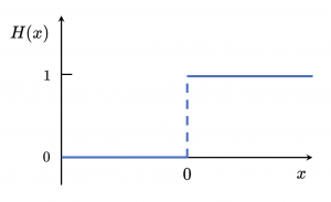
|
In evaluating this function at , we will adopt the half-maximum convention and set . As has been pointed out in, for example, a relevant Wikipedia discussion, the derivative of the unit step function is,
where, is the Dirac Delta function.
Perturbed Density
Let,
|
|
|
|
|
|
|
|
and, more generally after a perturbation, ,
|
|
|
|
Hence, in the linearized version of the continuity equation, we recognize that,
CORE:
|
|
|
|
and |
|
|
|
and |
|
|
|
ENVELOPE:
|
|
|
|
and |
|
|
|
and |
|
|
|
Perturbed Pressure
|
|
|
|
|
|
|
|
and, more generally after a perturbation, ,
|
|
|
|
Hence, in the linearized version of the first law of thermodynamics, we recognize that,
Obtaining Perturbed Density from Perturbed Pressure
Given that, quite generally,
|
|
|
|
let's define the density-like quantity,
in which case,
|
|
|
|
What happens if we perturb the pressure? In either region (core or envelope),
|
|
|
|
As a result,
|
|
|
|
|
|
|
|
|
|
|
|
|
|
|
|
|
|
|
|
|
|
|
|
Set of Linearized Equations
Borrowing from an accompanying discussion, we have …
|
Linearized
Equation of Continuity
Linearized
Euler + Poisson Equations
Linearized
Adiabatic Form of the
First Law of Thermodynamics
|
Rearranging terms in the "Linearized Euler + Poisson Equations" as follows …
|
|
|
|
we realize that the expression on the RHS has the same value at the interface, whether you're viewing the equation from the point of view of the core or the envelope; and we recognize as well that is a simple step function at the interface. Hence, letting a prime indicate differentiation with respect to , we can write,
|
|
|
|
Analogously, the "Linearized Equation of Continuity" can be rewritten as,
|
|
|
|
Now, given that , we see that,
|
|
|
|
and,
|
|
|
|
Hence, differentiation of the "Linearized Equation of Continuity" gives,
|
|
|
|
|
|
|
|
|
|
|
|
|
|
|
|
|
|
|
|
From the Perspective of the Core
When — that is, from the perspective of the core while including the interface,
|
|
|
|
|
|
|
|
And examining only the interface, where while ,
|
|
|
|
|
|
|
|
From the Perspective of the Envelope
When — that is, from the perspective of the envelope while including the interface,
|
|
|
|
|
|
|
|
Focus on Nonlinear Continuity Equation
A spherical shell of core density, , where the inner radius of the shell is and its outer radius is has a shell mass given by the expression,
|
|
|
|
|
|
|
|
|
|
|
|
|
|
|
|
|
|
|
|
|
|
|
|
Similarly, as viewed from the perspective of the envelope, it has a shell mass of,
|
|
|
|
|
|
|
|
Better yet, pick the two edges of the shell, and , and let and . Given the value of , the unperturbed mass in the shell is given by the above expression, that is,
|
|
|
|
Now, let and, . We then have,
|
|
|
|
|
|
|
|
|
|
|
|
|
|
|
|
|
|
|
|
In order for the shell to have the same in both the unperturbed and perturbed cases, the following relation must hold:
|
|
|
|
|
|
|
|
Work With Pair of First-Order Linearized Equations
Equilibrium Structures Using Preferred Normalizations
Working from our earlier "new" normalization — which was done in the context of our examination of the B-KB74 conjecture — that is, by setting,
|
New Normalization
|
|
|
|
|
|
|
|
|
|
|
|
|
|
|
|
and after adopting the notation,
|
|
|
(see definitions of , , and given below) we have throughout the core,
|
|
|
|
|
|
|
|
|
|
|
|
|
For later use, note that,
|
|
|
| |
|
|
| |
|
|
| |
|
|
Note as well that,
|
|
|
| |
|
|
| |
|
|
|
Similarly, throughout the envelope, we find,
|
|
|
|
|
|
|
|
|
|
|
|
|
|
|
|
where,
|
|
|
|
|
|
and,
|
|
|
|
|
|
|
|
|
|
|
|
|
|
|
|
|
|
Keep in mind, as well, that,
|
|
|
|
|
|
Linearized Equations With Preferred Normalizations
Review and Elaborate
|
Linearized
Equation of Continuity
Linearized
Euler + Poisson Equations
Linearized
Adiabatic Form of the
First Law of Thermodynamics
|
The LHS of the "linearized Euler + Poisson" equation is rewritten as,
|
|
|
| |
|
|
| |
|
|
and,
|
|
|
| |
|
|
| |
|
|
Therefore, multiplying the full equation through by gives,
|
|
|
| |
|
|
where the square of the characteristic timescale,
|
|
|
|
ASIDE: Building on an associated discussion, the square of the dimensionless frequency also can be represented by the expression,
|
|
|
where,
|
Hence we can write,
|
|
|
| |
|
|
Focusing on the core …
As demonstrated earlier, the leading term on the RHS of this expression can be rewritten to give,
|
|
|
|
|
|
Noting as well that,
|
|
|
we have,
|
|
|
At the Center
All σ2
According to our discussion in an appendix chapter, starting from the center of the equilibrium configuration, the displacement function can be represented by a power-series expression of the form,
where, , and (see, for example, here),
|
|
|
|
Note that, at the center of our bipolytrope, , so . Hence, for this particular investigation, the central boundary condition is,
|
|
|
|
|
|
|
|
Also, the derivative of this displacement function is,
Hence,
|
|
|
|
|
|
|
|
Furthermore, we find,
|
|
|
|
|
|
|
|
|
|
|
|
Hence we have,
|
|
|
| |
|
|
| |
|
|
| |
|
|
| |
|
|
Just σ2 = 0
If we set , we have,
|
|
|
|
|
|
|
|
Alternatively, from immediately above,
|
|
|
| |
|
|
| |
|
|
Yes! It matches!
Summary
Moving from the center, outward thorough the core — that is, interior to the interface — we can assign values of and using the following approximate (exact if ) relations:
|
|
|
|
|
|
|
|
For all radial shells throughout the entire bipolytropic configuration, the pair of first derivatives can be evaluated using the following relations:
|
|
|
|
|
|
|
Near the center, this pressure-derivative expression can be checked against the relation,
|
|
|
notice that, in order to make this comparison, you need to multiply this last expression through by the ratio,
|
|
|
The comparison should be especially accurate in the case of .
At the Interface
See below.
At the Surface
Drawing from a separate discussion, the surface boundary condition is,
|
|
|
at
|
that is,
|
|
|
|
where (see also, here),
Note that since,
|
|
|
|
in terms of our adopted normalizations, the frequency-squared term should be rewritten as,
|
|
|
|
Note as well that, at the surface of our bipolytrope, , so . Hence, for this particular investigation, the surface boundary condition is,
|
|
|
|
|
|
|
|
|
|
|
|
|
|
|
|
This result should be compared with our separate discussion of eigenfunction details.
Discretize for Numerical Integration
General Discretization
First Approximation
Now, let's set up a grid associated with a uniformly spaced spherical radius, where the subscript denotes the grid zone at which all terms in the finite-difference representation of the governing relations will be evaluated. More specifically,
|
|
|
and |
|
|
|
also,
|
|
|
and |
|
|
|
And at each grid location, the governing relations establish the local evaluation of the derivatives, that is,
|
|
|
and |
|
|
|
So, integrating step-by-step from the center of the configuration, outward, once all the variable values are known at grid locations and , the values of and at are given by the expressions,
|
|
|
and |
|
|
|
Then we will obtain the "" and "" values via the average expressions,
|
|
|
and |
|
|
|
|
Consider implementing a more implicit finite-difference analysis. Wherever a "" index appears in the source term, replace it with the average expressions. The general form of the source term expressions is,
|
|
|
| |
|
|
|
|
|
where,
|
|
|
and |
|
|
|
and,
|
|
|
| |
|
|
|
|
|
where,
|
|
|
and |
|
|
|
In both cases, the two unknowns are and . Combining this pair of equations gives,
|
|
|
|
|
|
which determines , which then allows the straightforward determination of . Via the average expressions, we can also then determine — and record — the self-consistent values of and .
Dropping terms and higher gives,
|
|
|
and, in turn,
|
|
|
|
Second Approximation
Let's assume that we know the three quantities, , and and want to project forward to determine, . We should assume that, locally, the displacement function is quadratic in , that is,
|
|
|
|
|
|
where we have three unknowns, . These can be determined by appropriately combining the three relations,
|
|
|
|
|
|
|
|
|
We have,
|
|
|
|
|
|
|
|
|
Combining the last two expressions gives,
|
|
|
|
|
|
|
|
|
|
|
|
Therefore, also,
|
|
|
|
|
|
Hence,
|
|
|
| |
|
|
| |
|
|
| |
|
|
| |
|
|
WRONG!! Try again …
Third Approximation
Let's assume that we know the three quantities, , and and want to project forward to determine, . We should assume that, locally, the displacement function is quadratic in , that is,
|
|
|
|
|
|
where we have three unknowns, . These can be determined by appropriately combining the three relations,
|
|
|
|
|
|
|
|
|
The difference between the last two expressions gives,
|
|
|
| |
|
|
Combining this with the first of the three expressions then gives,
|
|
|
|
|
|
|
|
|
|
|
|
|
|
|
|
Hence,
|
|
|
|
|
|
|
|
|
|
|
|
|
|
|
|
|
|
|
|
|
|
|
|
As a result,
|
|
|
| |
|
|
| |
|
|
| |
|
|
| |
|
|
| |
|
|
| |
|
|
| |
|
|
GOOD! This is the same as our first approximation expression stated above.
|
This is test ...
|
|
|
|
|
| 0.001936393 |
-4.695376 |
-4.547832 |
-116.0119 |
-76.19513 |
|
|
|
|
|
Part 2
For a continuation (part 2) of this discussion, go here.
See Also

