Apps/MaclaurinSpheroidSequence: Difference between revisions
| Line 1,206: | Line 1,206: | ||
</tr></table> | </tr></table> | ||
</td> | </td> | ||
</tr> | |||
</table> | |||
</li> | |||
</ol> | |||
---- | |||
<ol type="1" start="1983"> | |||
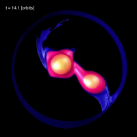
<li><div align="center">{{ EH83bfigure }}</div> | |||
<table border="1" align="center" cellpadding="5"> | |||
<tr> | |||
<td align="center">[[File:EH83bFig3.png|300px|EH83bFig3]]</td> | |||
<td align="center">[[File:EH83bFig4.png|200px|EH83bFig4]]</td> | |||
<td align="center">[[File:EH83bFig2.png|150px|EH83bFig2]]</td> | |||
</tr> | </tr> | ||
</table> | </table> | ||
Revision as of 16:40, 2 February 2023
Maclaurin Spheroid Sequence
| Maclaurin Spheroid Sequence |
|---|
Detailed Force Balance Conditions
Equilibrium Angular Velocity
| Figure 1 |
 |
|
The dark blue circular markers locate 15 of the 18 individual models identified in Table 1. The solid black curve derives from our evaluation of the function, this curve also may be found in: |
The essential structural elements of each Maclaurin spheroid model are uniquely determined once we specify the system's axis ratio, , or the system's meridional-plane eccentricity, , where
|
|
|
|
which varies from e = 0 (spherical structure) to e = 1 (infinitesimally thin disk). According to our accompanying derivation, for a given choice of , the square of the system's equilibrium angular velocity is,
|
|
|
|
|
[EFE], §32, p. 77, Eq. (4) |
||
where,
|
|
|
|
|
|
|
|
|
📚 Thomson & Tait (1867), §522, p. 392, Eqs. (9) & (7) |
||
| ||||||||||||||||||||||||||||||||||||||||||||||
In other words,
|
|
|
|
|
📚 Thomson & Tait (1867), §771, p. 613, Eq. (1) |
||
Figure 1 shows how the square of the angular velocity varies with eccentricity along the Maclaurin spheroid sequence; given the chosen normalization unit, , it is understood that the density of the configuration is held fixed as the eccentricity is varied.
| Examining the Maclaurin spheroid sequence "… we see that the value of increases gradually from zero to a maximum as the eccentricity rises from zero to about 0.93, and then (more quickly) falls to zero as the eccentricity rises from 0.93 to unity." … "If the angular velocity exceed the value associated with this maximum, "… equilibrium is impossible in the form of an ellipsoid of revolution. If the angular velocity fall short of this limit there are always two ellipsoids of revolution which satisfy the conditions of equilibrium. In one of these the eccentricity is greater than 0.93, in the other less." |
|
--- 📚 Thomson & Tait (1867), §772, p. 614. |
The extremum of the curve occurs where ; that is, it occurs where,
In our Figure 1, the small solid-green square marker identifies the location along the sequence where the system with the maximum angular velocity resides:
|
|
|
|
| [EFE], §32, p. 80, Eqs. (9) & (10) | ||
ASIDE
Suppose we set,
|
|
|
|
|
|
|
valid over the range, ; note, for example, that . Then we have,
|
|
|
|
|
|
|
|
|
|
|
|
|
|
|
|
|
|
|
|
|
|
|
|
|
Note, for example, that , in which case,
Plugging in the analytic expression for the eccentricity, we find,
Matches! |
Corresponding Total Angular Momentum
| Figure 2 |
 |
|
Solid black curve also may be found as: |
The total angular momentum of each uniformly rotating Maclaurin spheroid is given by the expression,
|
|
|
|
where, the moment of inertia and the total mass of a uniform-density spheroid are, respectively,
|
|
|
|
and, |
|
|
|
Hence, we have,
|
|
|
|
|
|
|
|
|
|
|
|
|
where, |
||
Figure 2 shows how the system's angular momentum varies with eccentricity along the Maclaurin spheroid sequence; given the chosen normalization unit, , it is understood that the mass and the volume — hence, also the density — of the configuration are held fixed as the eccentricity is varied. Strictly speaking, along this sequence the angular momentum asymptotically approaches infinity as ; by limiting the ordinate to a maximum value of 1.2, the plot masks this asymptotic behavior. The small solid-green square marker identifies the location along this sequence where the system with the maximum angular velocity resides (see Figure 1); this system is not associated with a turning point along this angular-momentum versus eccentricity sequence.
Alternate Sequence Diagrams
Energy Ratio, T/|W|
|
Table 2: Limiting Values |
||
|
|
|
|
|
|
|
|
|
|
|
|
|
|
|
|
|
|
|
|
The rotational kinetic energy of each uniformly rotating Maclaurin spheroid is given by the expression,
|
|
|
|
|
|
|
|
|
|
|
|
and the gravitational potential energy of each configuration is,
|
|
|
|
|
|
|
|
|
|
|
|
Hence, the energy ratio,
|
|
|
|
|
[T78], §4.5, p. 86, Eq. (53) |
||
|
|
|
|
|
|
|
|
|
[ST83], §7.3, p. 172, Eq. (7.3.24) |
||
Building on an accompanying discussion of the structure of Maclaurin spheroids, Table 2 — shown just above, on the right — lists the limiting values of several key functions. Note, in particular, that as the eccentricity varies smoothly from zero (spherical configuration) to unity (infinitesimally thin disk), the energy ratio, , varies smoothly from zero to one-half. In his examination of the Maclaurin spheroid sequence, Tassoul (1978) chose to use this energy ratio as the order parameter, rather than the eccentricity.
|


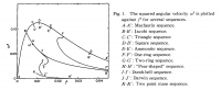
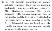
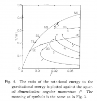
Following Tassoul, our Figure 3 shows how the square of the angular velocity varies with , and our Figure 4 shows how the system angular momentum varies with . In these plots, respectively, the square of the angular velocity has been normalized by — that is, by a quantity that is a factor of two larger than the normalization adopted in EFE — while the angular momentum has been normalized to the same quantity used in EFE. As above, the small solid-green square marker identifies the location along the sequence where the system with the maximum angular velocity resides.
Angular Velocity or T/|W| vs. Angular Momentum
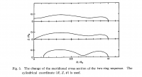
Figures 5 and 6, respectively, show how the square of the angular velocity and how the energy ratio, τ, vary with the square of the angular momentum for models along the Maclaurin spheroid sequence. In generating these plots, following the lead of Eriguchi & Hachisu (1983), we have normalized the square of the angular velocity by — a factor of four larger than the normalization used in EFE — and we have adopted a slightly different angular-momentum-squared normalization, namely,
|
|
|
|
|


As above, the small solid-green square marker identifies the location along both sequences where the system with the maximum angular velocity resides:
|
|
|
|
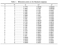
Bifurcation Points Along Maclaurin-Spheroid Sequence
Following the lead of Hachisu & Eriguchi (1984, PASJapan, 36, 497-503), let's shift to oblate-spheroidal coordinates which are related to Cartesian coordinates via the relations,
For axisymmetric configurations, such as Maclaurin spheroids, we also appreciate that,
In this coordinate system, the surface of the Maclaurin spheroid is marked by a specific value of the coordinate, — call it, — and points along the surface (in any meridional plane) are identified by varying from zero (equatorial plane) to unity (the pole). Given that the eccentricity of the spheroid is , we understand that,
|
|
||
|
|
Also, in order for the volume of the spheroid to remain constant — and equal to that of a sphere of the same total mass and density — along the sequence of spheroids we understand that,
|
|
||
|
|
||
|
|
||
|
|
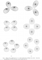
Models with Zero Vorticity when Viewed from Appropriate Rotating Frame
|


See Also
- Properties of Maclaurin Spheroids
- Excerpts from Maclaurin's (1742) A Treatise of Fluxions
- Properties of Homogeneous Ellipsoids
-
Equilibrium Configurations and Sequences Generated by Eriguchi, Hachisu, and their various colleagues:
- Y. Eriguchi & I. Hachisu (1982)
New Equilibrium Sequences Bifurcating from Maclaurin Sequence
Progress of Theoretical Physics, Vol. 67, No. 3, pp. 844 - 851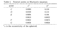
- Y. Eriguchi, I. Hachisu, & D. Sugimoto (1982)
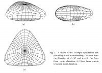
Dumb-Bell-Shape Equilibria and Mass-Shedding Pear-Shape
of Selfgravitating Incompressible Fluid
Progress of Theoretical Physics, Vol. 67, No. 4, pp. 1068 - 1075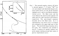
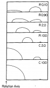
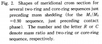
- Y. Eriguchi & I. Hachisu (1983a)
Two Kinds of Axially Symmetric Equilibrium Sequences of Self-Gravitating and Rotating Incompressible Fluid
— Two-Ring Sequence and Core-Ring Sequence —
Progress of Theoretical Physics, Vol. 69, No. 4, pp. 1131 - 1136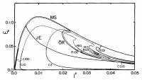
- Y. Eriguchi & I. Hachisu (1983b)
Gravitational Equilibrium of a Multi-Body Fluid System
Progress of Theoretical Physics, Vol. 70, No. 6, pp. 1534 - 1541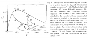
- I. Hachisu & Y. Eriguchi (1984)
Bifurcation Points on the Maclaurin Sequence
Publications of the Astronomical Society of Japan, Vol. 36, No. 3, pp. 497 - 503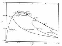


|
|---|
|
Appendices: | VisTrailsEquations | VisTrailsVariables | References | Ramblings | VisTrailsImages | myphys.lsu | ADS | |