Here we construct and analyze the relative stability of a bipolytrope in which the core has an polytropic index and the envelope has an polytropic index.
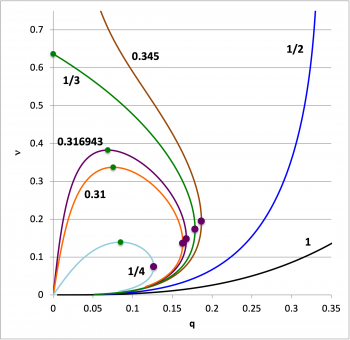
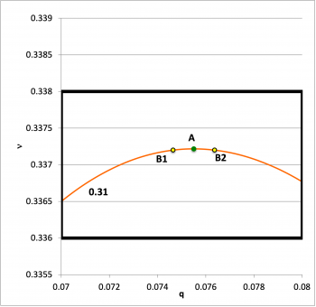
Maximum Fractional Core Mass, (solid green circular markers) for Equilibrium Sequences having Various Values of
LHS
RHS
---
---
---
---
---
---
---
0.0
0.0
0.33
24.00496
0.0719668
0.0710624
0.2128753
0.0726547
1.8516032
-223.8157
-223.8159
0.038378833
0.52024552
0.0
0.316943
10.744571
0.1591479
0.1493938
0.4903393
0.1663869
2.1760793
-31.55254
-31.55254
0.068652714
0.382383875
0.0
0.31
9.014959766
0.1886798
0.172320503
0.59835053
0.20081242
2.2823226
---
---
0.0755022550
0.3372170064
0.0
0.3090
8.8301772
0.1924833
0.1750954
0.6130669
0.2053811
2.2958639
-18.47809
-18.47808
0.076265588
0.331475715
0.0
4.9379256
0.3309933
0.2342522
1.4179907
0.4064595
2.761622
-2.601255
-2.601257
0.084824137
0.139370157
0.0
Recall that,
and
Also, go here for definition of , which identifies the location of the specific-entropy step function; stability against convection is ensured whenever .
We also have explored a "new normalization" based on holding and constant. Here we want to perform a Bonnor-Ebert-type analysis, examining how varies with radius if we hold and the core mass constant along an equilibrium sequence. According to our initial normalization — see, for example, here — we can write,
Therefore, from the analytic profiles that describe the core, we have,
we can flip from holding fixed to holding fixed via the relation,
As a result,
If we want to see the behavior along a sequence of the core mass, the expression is,
while the expression for the total mass is,
Summary: For fixed and
Stability
Introduction & Summary
Here we solve the LAWE numerically (on a uniformly zoned mesh — different for the separate core/envelope regions) using a 2nd-order accurate, implicit integration scheme in which the LAWE is broken into a pair of 1st-order ODEs. These results should be compared against a separate succinct discussion of our analysis obtained from integrating the LAWE in its standard 2nd-order ODE form.
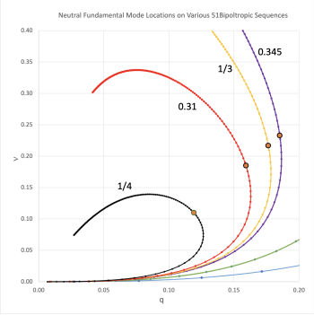
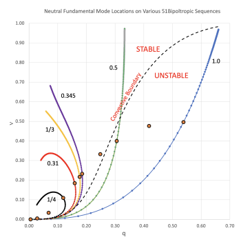
Properties of Neutral Fundamental Mode for Various Sequences
σc2 for Overtones
Ω2 for Overtones
1st
2nd
1st
2nd
1.000
1.6639103365
8.4811731
0.49622717
0.53833097
0.000000
2.528013
5.66087
10.72026
24.0054
0.500
2.2703111897
62.666493
0.399760079
0.305764976
0.000000
0.2659116
0.73022
8.33187
22.8802
0.345
2.546385206
205.77394
0.232779379
0.185262833
0.000000
0.06741185
0.198075
6.93580
20.3793
2.5675774773
225.75664
0.216806201
0.176420918
0.000000
0.0602615
0.178432
6.80222
20.1411
2.6095097538
270.59221
0.184909369
0.159274
0.000000
0.04821396
0.145248
6.52316
19.6515
2.712384289
415.67338
0.109935743
0.1192667
0.000000
0.02772424
0.088472
5.76211
18.3877
Model Sequence: μe/μc = 1.00
Marginally Unstable Model
Numbers presented in the following table should be compared against our earlier determinations. Various things to note:
As discussed elsewhere — for example, here — when , the radial displacement function for the core — that is, for all — should be given precisely by the expression,
Hence, given that ξi = 1.6639103365 as viewed from the perspective of the core, the magnitude of, and the logarithmic derivative of the radial displacement function should have the values, respectively,
and
As discussed elsewhere — for example, here — we expect,
file = Dropbox/WorkFolder/Wiki edits/BiPolytrope/TwoFirstOrderODEs/Bipolytrope51.xlsx --- worksheet = MuRatio100FundOur September 2023 Determinations for Marginally Unstable Model Having
NEW:
Mode
core
env
expected
measured
1 (Fundamental)
0.00
0.00
+0.81437470 0.8154268
-0.455872 -0.452703
-1.473523 -1.471622
+0.3820 0.3849493
-1
-0.999999992 -1.00618
n/a
n/a
n/a
n/a
n/a
n/a
2
2.51513333 2.528013
10.7107538 10.720258
0.20482050 0.2069746
-7.09124 -7.000803
-5.4547441 -5.400482
- 0.9962 -1.018215
4.355376917 4.360129
4.35537692 4.3999485
0.64133 0.6456
0.3502 0.3444
n/a
n/a
n/a
n/a
3
5.72371888 5.66087
24.3745901 24.0054
-0.14269277 -0.13587
+8.046019 +8.62053
+3.627611 +3.9723
+0.9308 +0.98810
11.18729505 11.0027
11.18729506 11.8164
0.4837 0.48395
0.5864 0.58326
0.842 0.84145
0.0854 0.08576
n/a
n/a
4
10.3458476
44.0622916
-0.20845197
-0.6949966
-1.61699793
-1.1443
21.03114578
21.03114577
0.3939
0.7154
0.6902
0.2777
0.9115
0.0284
Model Sequence: μe/μc = 0.31
Here we examine how the frequency of the 1st overtone varies as is increased.
Frequency Variation Along the Sequence having
Note
1st Overtone
Fundamental
1.6
58.39858647
0.498473
14.5550593
0.1333725
3.8943827
2.0000
108.69129
0.236047
12.82812694
0.07011655
3.8105293
2.4000
199.16363
0.0870005
8.6636677
0.028066485
2.794911541
Neutral Fundamental ==>
2.6095097538
270.5922
0.04821396
6.523161
0.0
0.0
3.0000
468.1500
0.02329066
5.451761
-0.056763527
-13.2869232
3.5
902.640279
0.011747773
5.302006549
- 0.098905428
-44.63801154
4.0000
1656.926
0.006427613
5.325041
-0.118551256677297
-98.21535777
5.0000
4900.105
0.002215415
5.4279
---
---
6.0000
12544.67
0.000878472
5.510074
---
---
==>
9.014959766
5.60367789
---
---
12.0000
5.579608
---
---
SearchMuRatio
Adding models to the above table, here we choose and iterate until we have found the value of that corresponds to the fundamental-mode. At the interface, we expect,
Throughout the core, for the neutral (i.e., ) fundamental mode of oscillation, we expect that,
Given that at the interface, we expect,
Similarly at the surface of the envelope for the neutral (i.e., ) fundamental mode of oscillation, we expect that,
file = Dropbox/WorkFolder/Wiki edits/BiPolytrope/TwoFirstOrderODEs/Bipolytrope51New.xlsx --- worksheet = ConvectiveBoundaryProperties of Neutral Fundamental Mode for Various Sequences