SSC/Stability/BiPolytropes/51Models: Difference between revisions
| (86 intermediate revisions by the same user not shown) | |||
| Line 21: | Line 21: | ||
<table border="1" align="center" cellpadding="8"> | <table border="1" align="center" cellpadding="8"> | ||
<tr> | <tr> | ||
<td align="center" colspan=" | <td align="center" colspan="13"> | ||
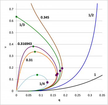
<b>Maximum Fractional Core Mass, <math>\nu = M_\mathrm{core}/M_\mathrm{tot}</math> (solid green circular markers)<br />for Equilibrium Sequences having Various Values of <math>\mu_e/\mu_c</math> | <b>Maximum Fractional Core Mass, <math>\nu = M_\mathrm{core}/M_\mathrm{tot}</math> (solid green circular markers)<br />for Equilibrium Sequences having Various Values of <math>\mu_e/\mu_c</math> | ||
</td> | </td> | ||
| Line 59: | Line 59: | ||
<math>\nu \equiv \frac{M_\mathrm{core}}{M_\mathrm{tot}}</math> | <math>\nu \equiv \frac{M_\mathrm{core}}{M_\mathrm{tot}}</math> | ||
</td> | </td> | ||
<td align="right"> | |||
<math>[\xi_i]_\mathrm{smooth}</math> </td> | |||
<td align="center" rowspan="7">[[File:TurningPoints51BipolytropesLabels.png|450px|Extrema along Various Equilibrium Sequences]]</td> | <td align="center" rowspan="7">[[File:TurningPoints51BipolytropesLabels.png|450px|Extrema along Various Equilibrium Sequences]]</td> | ||
</tr> | </tr> | ||
| Line 78: | Line 80: | ||
<td align="center"> | <td align="center"> | ||
<math>\frac{2}{\pi}</math> </td> | <math>\frac{2}{\pi}</math> </td> | ||
<td align="right"> | |||
0.0 </td> | |||
</tr> | </tr> | ||
| Line 104: | Line 108: | ||
<td align="right"> | <td align="right"> | ||
0.52024552 </td> | 0.52024552 </td> | ||
<td align="right"> | |||
0.0 </td> | |||
</tr> | </tr> | ||
| Line 130: | Line 136: | ||
<td align="right"> | <td align="right"> | ||
0.382383875 </td> | 0.382383875 </td> | ||
<td align="right"> | |||
0.0 </td> | |||
</tr> | </tr> | ||
| Line 139: | Line 147: | ||
9.014959766 </td> | 9.014959766 </td> | ||
<td align="center"> | <td align="center"> | ||
0.1886798 </td> | |||
<td align="center"> | <td align="center"> | ||
0.172320503 </td> | |||
<td align="right"> | <td align="right"> | ||
0.59835053 </td> | 0.59835053 </td> | ||
<td align="center"> | <td align="center"> | ||
0.20081242 </td> | |||
<td align="center"> | <td align="center"> | ||
2.2823226 </td> | |||
<td align="center"> | <td align="center"> | ||
--- </td> | --- </td> | ||
| Line 156: | Line 164: | ||
<td align="right"> | <td align="right"> | ||
0.3372170064 </td> | 0.3372170064 </td> | ||
<td align="right"> | |||
0.0 </td> | |||
</tr> | </tr> | ||
| Line 182: | Line 192: | ||
<td align="right"> | <td align="right"> | ||
0.331475715 </td> | 0.331475715 </td> | ||
<td align="right"> | |||
0.0 </td> | |||
</tr> | </tr> | ||
| Line 208: | Line 220: | ||
<td align="right"> | <td align="right"> | ||
0.139370157 </td> | 0.139370157 </td> | ||
<td align="right"> | |||
0.0 </td> | |||
</tr> | </tr> | ||
<tr> | <tr> | ||
<td align="left" colspan=" | <td align="left" colspan="13"> | ||
Recall that, | Recall that, | ||
<div align="center"> | <div align="center"> | ||
| Line 222: | Line 236: | ||
</math> | </math> | ||
</div> | </div> | ||
Also, go [[Appendix/Ramblings/PatrickMotl#Pick_a_Different_Molecular-Weight_Ratio|here]] for definition of <math>[\xi_i]_\mathrm{smooth}</math>, which identifies the location of the specific-entropy step function; stability against convection is ensured whenever <math>\xi_i > [\xi_i]_\mathrm{smooth}</math>. | |||
</td> | </td> | ||
</tr> | </tr> | ||
| Line 277: | Line 292: | ||
<td align="center">[[File:TurningPoints51BipolytropesLabels.png|right|350px|Bipolytropic (5, 1) Equilibrium Sequences]]</td> | <td align="center">[[File:TurningPoints51BipolytropesLabels.png|right|350px|Bipolytropic (5, 1) Equilibrium Sequences]]</td> | ||
<td align="center">[[File:TurningPoints51Bpairing.png|right|350px|Bipolytropic (5, 1) Equilibrium Sequences]]</td> | <td align="center">[[File:TurningPoints51Bpairing.png|right|350px|Bipolytropic (5, 1) Equilibrium Sequences]]</td> | ||
</tr> | |||
</table> | |||
<table border="1" align="center" cellpadding="10"> | |||
<tr> | |||
<td align="center">[[File:FundModeLocations02Labels.png|right|350px|Bipolytropic (5, 1) Neutral Fundamental Mode Locations]]</td> | |||
<td align="center">[[File:ConvectiveBoundary2Labeled.png|right|350px|Bipolytropic (5, 1) Equilibrium Sequences]]</td> | |||
</tr> | </tr> | ||
</table> | </table> | ||
| Line 284: | Line 306: | ||
</li> | </li> | ||
</ol> | </ol> | ||
==Yet Another Normalization== | |||
===Fixed Core Mass=== | |||
Initially, our normalization was based on [[SSC/Structure/BiPolytropes/Analytic51#Normalization|holding <math>K_c</math> and the central density <math>(\rho_0)</math> constant]]. Specifically, | |||
<table border="0" cellpadding="3" align="center"> | |||
<tr> | |||
<td align="right"> | |||
<math>\rho^*</math> | |||
</td> | |||
<td align="center"> | |||
<math>\equiv</math> | |||
</td> | |||
<td align="left"> | |||
<math>\frac{\rho}{\rho_0}</math> | |||
</td> | |||
<td align="center">; </td> | |||
<td align="right"> | |||
<math>r^*</math> | |||
</td> | |||
<td align="center"> | |||
<math>\equiv</math> | |||
</td> | |||
<td align="left"> | |||
<math>\frac{r}{[K_c^{1/2}/(G^{1/2}\rho_0^{2/5})]}</math> | |||
</td> | |||
</tr> | |||
<tr> | |||
<td align="right"> | |||
<math>P^*</math> | |||
</td> | |||
<td align="center"> | |||
<math>\equiv</math> | |||
</td> | |||
<td align="left"> | |||
<math>\frac{P}{K_c\rho_0^{6/5}}</math> | |||
</td> | |||
<td align="center">; </td> | |||
<td align="right"> | |||
<math>M_r^*</math> | |||
</td> | |||
<td align="center"> | |||
<math>\equiv</math> | |||
</td> | |||
<td align="left"> | |||
<math>\frac{M_r}{[K_c^{3/2}/(G^{3/2}\rho_0^{1/5})]}</math> | |||
</td> | |||
</tr> | |||
<tr> | |||
<td align="right"> | |||
<math>H^*</math> | |||
</td> | |||
<td align="center"> | |||
<math>\equiv</math> | |||
</td> | |||
<td align="left"> | |||
<math>\frac{H}{K_c\rho_0^{1/5}}</math> | |||
</td> | |||
<td align="center">. </td> | |||
<td align="right" colspan="3"> | |||
| |||
</td> | |||
</tr> | |||
</table> | |||
We also have explored a [[SSC/Structure/BiPolytropes/51RenormaizePart2#Basic_Equilibrium_Structure|"new normalization"]] based on holding <math>K_c</math> and <math>M_\mathrm{tot}</math> constant. Here we want to perform a Bonnor-Ebert-type analysis, examining how <math>P_i</math> varies with radius if we hold <math>K_c</math> and the ''core mass'' constant along an equilibrium sequence. According to our initial normalization — see, for example, [[SSC/Structure/BiPolytropes/Analytic51Renormalize#Step_4:_Throughout_the_core|here]] — we can write, | |||
<table border="0" cellpadding="3" align="center"> | |||
<tr> | |||
<td align="right"> | |||
<math>M_\mathrm{core}</math> | |||
</td> | |||
<td align="center"> | |||
<math>=</math> | |||
</td> | |||
<td align="left"> | |||
<math>\biggl[ \frac{K_c^3}{G^3 \rho_0^{2/5} } \biggr]^{1/2} \biggl( \frac{2\cdot 3}{\pi } \biggr)^{1/2} ( \xi_i \theta_i )^3</math> | |||
</td> | |||
</tr> | |||
<tr> | |||
<td align="right"> | |||
<math>\Rightarrow ~~~ \rho_0^{1 / 5}</math> | |||
</td> | |||
<td align="center"> | |||
<math>=</math> | |||
</td> | |||
<td align="left"> | |||
<math>\biggl[ \frac{K_c^3}{G^3 M_\mathrm{core}^2 } \biggr]^{1/2} \biggl( \frac{2\cdot 3}{\pi } \biggr)^{1/2} ( \xi_i \theta_i )^3</math> | |||
</td> | |||
</tr> | |||
</table> | |||
Therefore, from the analytic profiles that describe the core, we have, | |||
<table border="0" cellpadding="3" align="center"> | |||
<tr> | |||
<td align="right"> | |||
<math>\rho_i</math> | |||
</td> | |||
<td align="center"> | |||
<math>=</math> | |||
</td> | |||
<td align="left"> | |||
<math>\rho_0 \theta_i^5</math> | |||
</td> | |||
<td align="center"> | |||
<math>=</math> | |||
</td> | |||
<td align="left"> | |||
<math>\rho_0 \theta_i^5</math> | |||
</td> | |||
</tr> | |||
<tr> | |||
<td align="right"> | |||
<math>P</math> | |||
</td> | |||
<td align="center"> | |||
<math>=</math> | |||
</td> | |||
<td align="left"> | |||
<math>K_c \rho_0^{6/5} \theta_i^6</math> | |||
</td> | |||
<td align="center"> | |||
<math>=</math> | |||
</td> | |||
<td align="left"> | |||
<math>K_c \rho_0^{6/5} \theta_i^6</math> | |||
</td> | |||
</tr> | |||
<tr> | |||
<td align="right"> | |||
<math>r</math> | |||
</td> | |||
<td align="center"> | |||
<math>=</math> | |||
</td> | |||
<td align="left"> | |||
<math>\biggl[ \frac{K_c}{G\rho_0^{4/5}} \biggr]^{1/2} \biggl(\frac{3}{2\pi}\biggr)^{1/2} \xi_i</math> | |||
</td> | |||
<td align="center"> | |||
<math>=</math> | |||
</td> | |||
<td align="left"> | |||
<math>\biggl[ \frac{K_c}{G\rho_0^{4/5}} \biggr]^{1/2} \biggl(\frac{3}{2\pi}\biggr)^{1/2} \xi_i</math> | |||
</td> | |||
</tr> | |||
<tr> | |||
<td align="right"> | |||
<math>M_i</math> | |||
</td> | |||
<td align="center"> | |||
<math>=</math> | |||
</td> | |||
<td align="left"> | |||
<math>\biggl[ \frac{K_c^3}{G^3 \rho_0^{2/5} } \biggr]^{1/2} \biggl( \frac{2\cdot 3}{\pi } \biggr)^{1/2} ( \xi_i \theta_i)^3 </math> | |||
</td> | |||
<td align="center"> | |||
<math>=</math> | |||
</td> | |||
<td align="left"> | |||
<math>\biggl[ \frac{K_c^3}{G^3 \rho_0^{2/5} } \biggr]^{1/2} \biggl( \frac{2\cdot 3}{\pi } \biggr)^{1/2} ( \xi_i \theta_i)^3 </math> | |||
</td> | |||
</tr> | |||
</table> | |||
<table border="0" align="center" cellpadding="5"> | |||
<tr> | |||
<td align="right"><math>\rho_i</math></td> | |||
<td align="center"><math>=</math></td> | |||
<td align="left"> | |||
<math> | |||
\rho_0 \theta_i^5 | |||
</math> | |||
</td> | |||
</tr> | |||
<tr> | |||
<td align="right"> </td> | |||
<td align="center"><math>=</math></td> | |||
<td align="left"> | |||
<math> | |||
\biggl\{ | |||
\biggl[ \frac{K_c^3}{G^3 M_\mathrm{core}^2 } \biggr]^{1/2} \biggl( \frac{2\cdot 3}{\pi } \biggr)^{1/2} ( \xi_i \theta_i )^3 | |||
\biggr\}^5 \theta_i^5 | |||
</math> | |||
</td> | |||
</tr> | |||
<tr> | |||
<td align="right"> </td> | |||
<td align="center"><math>=</math></td> | |||
<td align="left"> | |||
<math> | |||
\biggl[ \frac{K_c^3}{G^3 M_\mathrm{core}^2 } \biggr]^{5/2} \biggl( \frac{2\cdot 3}{\pi } \biggr)^{5/2} \xi_i^{15} \theta_i^{20} \, , | |||
</math> | |||
</td> | |||
</tr> | |||
<tr> | |||
<td align="right"><math>P_i</math></td> | |||
<td align="center"><math>=</math></td> | |||
<td align="left"> | |||
<math> | |||
K_c \rho_0^{6/5} \theta_i^6 | |||
</math> | |||
</td> | |||
</tr> | |||
<tr> | |||
<td align="right"> </td> | |||
<td align="center"><math>=</math></td> | |||
<td align="left"> | |||
<math> | |||
K_c\biggl\{ | |||
\biggl[ \frac{K_c^3}{G^3 M_\mathrm{core}^2 } \biggr]^{1/2} \biggl( \frac{2\cdot 3}{\pi } \biggr)^{1/2} ( \xi_i \theta_i )^3 | |||
\biggr\}^6 \theta_i^6 | |||
</math> | |||
</td> | |||
</tr> | |||
<tr> | |||
<td align="right"> </td> | |||
<td align="center"><math>=</math></td> | |||
<td align="left"> | |||
<math> | |||
\biggl[ \frac{K_c^{10}}{G^9 M_\mathrm{core}^6 } \biggr] \biggl( \frac{2\cdot 3}{\pi } \biggr)^{3} \xi_i^{18} \theta_i^{24} \, , | |||
</math> | |||
</td> | |||
</tr> | |||
<tr> | |||
<td align="right"><math>r_i</math></td> | |||
<td align="center"><math>=</math></td> | |||
<td align="left"> | |||
<math> | |||
\biggl[ \frac{K_c}{G\rho_0^{4/5}} \biggr]^{1/2} \biggl(\frac{3}{2\pi}\biggr)^{1/2} \xi_i | |||
</math> | |||
</td> | |||
</tr> | |||
<tr> | |||
<td align="right"> </td> | |||
<td align="center"><math>=</math></td> | |||
<td align="left"> | |||
<math> | |||
\biggl[ \frac{K_c}{G}\biggr]^{1/2} \biggl\{ | |||
\biggl[ \frac{K_c^3}{G^3 M_\mathrm{core}^2 } \biggr]^{1/2} \biggl( \frac{2\cdot 3}{\pi } \biggr)^{1/2} ( \xi_i \theta_i )^3 | |||
\biggr\}^{-2} \biggl(\frac{3}{2\pi}\biggr)^{1/2} \xi_i | |||
</math> | |||
</td> | |||
</tr> | |||
<tr> | |||
<td align="right"> </td> | |||
<td align="center"><math>=</math></td> | |||
<td align="left"> | |||
<math> | |||
\biggl[ \frac{G}{K_c}\biggr]^{5/2} M_\mathrm{core}^{-1} | |||
\biggl(\frac{\pi}{2^3 3}\biggr)^{1/2} \xi_i^{-5} \theta_i^{-6} | |||
</math> | |||
</td> | |||
</tr> | |||
<tr> | |||
<td align="right"><math>\Rightarrow ~~~ \mathrm{volume}~=\biggl(\frac{2^2\pi}{3}\biggr)r_i^3</math></td> | |||
<td align="center"><math>=</math></td> | |||
<td align="left"> | |||
<math> | |||
\biggl(\frac{2^2\pi}{3}\biggr)\biggl\{ | |||
\biggl[ \frac{G}{K_c}\biggr]^{5/2} M_\mathrm{core}^{-1} | |||
\biggl(\frac{\pi}{2^3 3}\biggr)^{1/2} \xi_i^{-5} \theta_i^{-6} | |||
\biggr\}^3 | |||
</math> | |||
</td> | |||
</tr> | |||
<tr> | |||
<td align="right"> </td> | |||
<td align="center"><math>=</math></td> | |||
<td align="left"> | |||
<math> | |||
\biggl[ \frac{G}{K_c}\biggr]^{15/2} M_\mathrm{core}^{-3} | |||
\biggl(\frac{\pi}{2 \cdot 3}\biggr)^{5/2} | |||
\xi_i^{-15} \theta_i^{-18} \, , | |||
</math> | |||
</td> | |||
</tr> | |||
<tr> | |||
<td align="right"><math>M_i</math></td> | |||
<td align="center"><math>=</math></td> | |||
<td align="left"> | |||
<math> | |||
\biggl[ \frac{K_c^3}{G^3 \rho_0^{2/5} } \biggr]^{1/2} \biggl( \frac{2\cdot 3}{\pi } \biggr)^{1/2} ( \xi_i \theta_i)^3 | |||
</math> | |||
</td> | |||
</tr> | |||
<tr> | |||
<td align="right"> </td> | |||
<td align="center"><math>=</math></td> | |||
<td align="left"> | |||
<math> | |||
\biggl[ \frac{K_c^3}{G^3 } \biggr]^{1/2} \biggl( \frac{2\cdot 3}{\pi } \biggr)^{1 / 2} | |||
\biggl\{ | |||
\biggl[ \frac{K_c^3}{G^3 M_\mathrm{core}^2 } \biggr]^{1/2} \biggl( \frac{2\cdot 3}{\pi } \biggr)^{1/2} ( \xi_i \theta_i )^3 | |||
\biggr\}^{-1} ( \xi_i \theta_i)^3 | |||
</math> | |||
</td> | |||
</tr> | |||
<tr> | |||
<td align="right"> </td> | |||
<td align="center"><math>=</math></td> | |||
<td align="left"> | |||
<math> | |||
M_\mathrm{core} \, . | |||
</math> | |||
</td> | |||
</tr> | |||
</table> | |||
Immediately below we reproduce [[SSC/Structure/PolytropesEmbedded#Fig3|Figure 3 from our accompanying discussion of ''embedded (pressure-truncated) polytropes'' having <math>n=5</math>]]. Notice that frame (a) contains a plot that displays our "yet another normalization" expressions for <math>P_i</math> vs. volume. | |||
<div align="center" id="Fig3"> | |||
<table border="1" align="center" cellpadding="8" width="1050px"> | |||
<tr> | |||
<td align="center" colspan="6"> | |||
Equilibrium Sequences of Pressure-Truncated, n = 5 Polytropic Spheres<br />(viewed from several different astrophysical perspectives) | |||
</td> | |||
</tr> | |||
<tr> | |||
<td align="center"><font color="black" size="+2">●</font></td><td align="center"><math>~\xi_e</math></td> | |||
<td align="center" width="300px"><sup>†</sup>External Pressure vs. Volume<br /><font size="-1">(Fixed Mass)</font></td> | |||
<td align="center" width="300px">Mass vs. Radius<br /><font size="-1">(Fixed External Pressure)</font></td> | |||
<td align="center" width="300px"><sup>‡</sup>Mass vs. Central Density<br /><font size="-1">(Fixed External Pressure)</font></td> | |||
<td align="center" width="300px">Mass vs. Central Density<br /><font size="-1">(Fixed Radius)</font></td> | |||
</tr> | |||
<tr> | |||
<td align="center" colspan="1"><font color="yellow" size="+2">●</font></td> <td align="center" colspan="1">√3</td> | |||
<td align="center" colspan="1" rowspan="4">(a)<br /> | |||
[[File:N5Sequence01B.png|300px|center|Pressure-Truncated Isothermal Equilibrium Sequence]] | |||
</td> | |||
<td align="center" colspan="1" rowspan="4">(b)<br /> | |||
[[File:N5Sequence02B.png|300px|center|Pressure-Truncated Isothermal Equilibrium Sequence]] | |||
</td> | |||
<td align="center" colspan="1" rowspan="4">(c)<br /> | |||
[[File:N5Sequence03B.png|300px|center|Pressure-Truncated Isothermal Equilibrium Sequence]] | |||
</td> | |||
<td align="center" colspan="1" rowspan="4">(d)<br /> | |||
[[File:N5Sequence04B.png|300px|center|Pressure-Truncated Isothermal Equilibrium Sequence]] | |||
</td> | |||
</tr> | |||
<tr> | |||
<td align="center" colspan="1"><font color="darkgreen" size="+2">●</font></td> <td align="center" colspan="1">3</td> | |||
</tr> | |||
<tr> | |||
<td align="center" colspan="1"><font color="purple" size="+2">●</font></td> <td align="center" colspan="1">√15</td> | |||
</tr> | |||
<tr> | |||
<td align="center" colspan="1"><font color="red" size="+2">●</font></td> <td align="center" colspan="1">9.01</td> | |||
</tr> | |||
<tr> | |||
<td align="center" colspan="2"> </td> | |||
<td align="center" colspan="1"><math>\biggl(\frac{2\cdot 3}{\pi}\biggr)^3 \biggl[ \xi^{18} \biggl(1 + \frac{\xi^2}{3} \biggr)^{-12} \biggr]_\tilde\xi</math><br /> vs. <br /> | |||
<math>\biggl(\frac{\pi}{2\cdot 3}\biggr)^{5/2} \biggl[ \xi^{-15} \biggl(1 + \frac{\xi^2}{3} \biggr)^{9}\biggr]_\tilde\xi</math> | |||
</td> | |||
<td align="center" colspan="1"><math>\biggl(\frac{2\cdot 3}{\pi}\biggr)^{1 / 2}\biggl[ \xi^{3} \biggl(1 + \frac{\xi^2}{3} \biggr)^{-2}\biggr]_\tilde\xi</math> <br /> vs. | |||
<br /> <math>\biggl(\frac{3}{2\pi}\biggr)^{1 / 2} \biggl[ \xi \biggl(1 + \frac{\xi^2}{3} \biggr)^{-1} \biggr]_\tilde\xi</math></td> | |||
<td align="center" colspan="1"><math>\biggl(\frac{2\cdot 3}{\pi}\biggr)^{1 / 2} \biggl[ \xi^{3} \biggl(1 + \frac{\xi^2}{3} \biggr)^{-2}\biggr]_\tilde\xi</math> <br /> vs. <br /> <math>\biggl[ \biggl(1 + \frac{\xi^2}{3} \biggr)^{5/2}\biggr]_\tilde\xi</math> | |||
</td> | |||
<td align="center" colspan="1"><math>\biggl[ \frac{2^3\cdot 3}{\pi} \biggr]^{1 / 4} \biggl[ \xi^{5/2}\biggl(1 + \frac{\xi^2}{3}\biggr)^{-3 / 2}\biggr]_\tilde\xi</math> <br /> vs. <br /> <math>\biggl[ \frac{3}{2\pi} \biggr]^{5 / 4} \tilde\xi^{5 / 2}</math> | |||
</td> | |||
</tr> | |||
</table> | |||
</div> | |||
===Fixed Radius=== | |||
Given that … | |||
<table border="0" cellpadding="3" align="center"> | |||
<tr> | |||
<td align="right"> | |||
<math>\rho^*</math> | |||
</td> | |||
<td align="center"> | |||
<math>\equiv</math> | |||
</td> | |||
<td align="left"> | |||
<math>\frac{\rho}{\rho_0}</math> | |||
</td> | |||
<td align="center">; </td> | |||
<td align="right"> | |||
<math>r^*</math> | |||
</td> | |||
<td align="center"> | |||
<math>\equiv</math> | |||
</td> | |||
<td align="left"> | |||
<math>\frac{r}{[K_c^{1/2}/(G^{1/2}\rho_0^{2/5})]}</math> | |||
</td> | |||
</tr> | |||
<tr> | |||
<td align="right"> | |||
<math>P^*</math> | |||
</td> | |||
<td align="center"> | |||
<math>\equiv</math> | |||
</td> | |||
<td align="left"> | |||
<math>\frac{P}{K_c\rho_0^{6/5}}</math> | |||
</td> | |||
<td align="center">; </td> | |||
<td align="right"> | |||
<math>M_r^*</math> | |||
</td> | |||
<td align="center"> | |||
<math>\equiv</math> | |||
</td> | |||
<td align="left"> | |||
<math>\frac{M_r}{[K_c^{3/2}/(G^{3/2}\rho_0^{1/5})]}</math> | |||
</td> | |||
</tr> | |||
<tr> | |||
<td align="right"> | |||
<math>H^*</math> | |||
</td> | |||
<td align="center"> | |||
<math>\equiv</math> | |||
</td> | |||
<td align="left"> | |||
<math>\frac{H}{K_c\rho_0^{1/5}}</math> | |||
</td> | |||
<td align="center">. </td> | |||
<td align="right" colspan="3"> | |||
| |||
</td> | |||
</tr> | |||
</table> | |||
we can flip from holding <math>\rho_0</math> fixed to holding <math>R</math> fixed via the relation, | |||
<table border="0" align="center" cellpadding="5"> | |||
<tr> | |||
<td align="right"><math>R = [K_c^{1/2}/(G^{1/2}\rho_0^{2/5})]R^*</math></td> | |||
<td align="center"><math>=</math></td> | |||
<td align="left"> | |||
<math>\biggl[ \frac{K_c}{(G\rho_0^{4/5})}\biggr]^{1 / 2} | |||
\biggl(\frac{1}{2\pi}\biggr)^{1 / 2} \biggl(\frac{\mu_e}{\mu_c}\biggr)^{-1} \frac{\eta_s}{\theta_i^2} | |||
</math> | |||
</td> | |||
</tr> | |||
<tr> | |||
<td align="right"><math>\Rightarrow ~~~ R^2</math></td> | |||
<td align="center"><math>=</math></td> | |||
<td align="left"> | |||
<math>\biggl[ \frac{K_c}{G\rho_0^{4/5}}\biggr] | |||
\biggl(\frac{1}{2\pi}\biggr) \biggl(\frac{\mu_e}{\mu_c}\biggr)^{-2} \eta_s^2 \theta_i^{-4} | |||
</math> | |||
</td> | |||
</tr> | |||
<tr> | |||
<td align="right"><math>\Rightarrow ~~~ \rho_0^{4 / 5}</math></td> | |||
<td align="center"><math>=</math></td> | |||
<td align="left"> | |||
<math> | |||
\biggl[ \frac{K_c}{GR^2}\biggr] | |||
\biggl(\frac{1}{2\pi}\biggr) \biggl(\frac{\mu_e}{\mu_c}\biggr)^{-2} \eta_s^2 \theta_i^{-4} | |||
</math> | |||
</td> | |||
</tr> | |||
</table> | |||
As a result, | |||
<table border="0" align="center" cellpadding="5"> | |||
<tr> | |||
<td align="right"><math>M = [K_c^{3 /2}/(G^{3 /2}\rho_0^{1/5})]M^*</math></td> | |||
<td align="center"><math>=</math></td> | |||
<td align="left"> | |||
<math> | |||
\biggl[ \frac{K_c^{3}}{G^{3}\rho_0^{2/5}}\biggr]^{1 / 2}M^*</math> | |||
</td> | |||
</tr> | |||
<tr> | |||
<td align="right"><math>\Rightarrow~~~ M^4</math></td> | |||
<td align="center"><math>=</math></td> | |||
<td align="left"> | |||
<math> | |||
\biggl[ \frac{K_c^{6}}{G^{6}}\biggr]\rho_0^{-4 / 5}(M^*)^4</math> | |||
</td> | |||
</tr> | |||
<tr> | |||
<td align="right"> </td> | |||
<td align="center"><math>=</math></td> | |||
<td align="left"> | |||
<math> | |||
\biggl[ \frac{K_c^{6}}{G^{6}}\biggr]\biggl\{ | |||
\biggl[ \frac{K_c}{GR^2}\biggr] | |||
\biggl(\frac{1}{2\pi}\biggr) \biggl(\frac{\mu_e}{\mu_c}\biggr)^{-2} \eta_s^2 \theta_i^{-4} | |||
\biggr\}^{-1}(M^*)^4</math> | |||
</td> | |||
</tr> | |||
<tr> | |||
<td align="right"> </td> | |||
<td align="center"><math>=</math></td> | |||
<td align="left"> | |||
<math> | |||
2\pi \biggl[ \frac{K_c^{5}R^2}{G^{5}}\biggr] | |||
\biggl(\frac{\mu_e}{\mu_c}\biggr)^{2} \eta_s^{-2} \theta_i^{4} | |||
(M^*)^4 \, .</math> | |||
</td> | |||
</tr> | |||
</table> | |||
If we want to see the behavior along a sequence of the core mass, the expression is, | |||
<table border="0" align="center" cellpadding="5"> | |||
<tr> | |||
<td align="right"><math>M_\mathrm{core}^4</math></td> | |||
<td align="center"><math>=</math></td> | |||
<td align="left"> | |||
<math> | |||
2\pi \biggl[ \frac{K_c^{5}R^2}{G^{5}}\biggr] | |||
\biggl(\frac{\mu_e}{\mu_c}\biggr)^{2} \eta_s^{-2} \theta_i^{4} | |||
\biggl[ | |||
\biggl(\frac{6}{\pi}\biggr)^{1 / 2} \xi_i^3 \theta_i^3 | |||
\biggr]^4 </math> | |||
</td> | |||
</tr> | |||
<tr> | |||
<td align="right"> </td> | |||
<td align="center"><math>=</math></td> | |||
<td align="left"> | |||
<math> | |||
\biggl(\frac{2^3\cdot 3^2}{\pi}\biggr) \biggl[ \frac{K_c^{5}R^2}{G^{5}}\biggr] | |||
\biggl(\frac{\mu_e}{\mu_c}\biggr)^{2} \eta_s^{-2} | |||
\biggl[ | |||
\xi_i^{12} \theta_i^{16} | |||
\biggr] \, ;</math> | |||
</td> | |||
</tr> | |||
</table> | |||
while the expression for the total mass is, | |||
<table border="0" align="center" cellpadding="5"> | |||
<tr> | |||
<td align="right"><math>M_\mathrm{tot}^4</math></td> | |||
<td align="center"><math>=</math></td> | |||
<td align="left"> | |||
<math> | |||
2\pi \biggl[ \frac{K_c^{5}R^2}{G^{5}}\biggr] | |||
\biggl(\frac{\mu_e}{\mu_c}\biggr)^{2} \eta_s^{-2} \theta_i^{4} | |||
\biggl[ | |||
\biggl(\frac{\mu_e}{\mu_c}\biggr)^{-2}\biggl(\frac{2}{\pi}\biggr)^{1 / 2} A\eta_s \theta_i^{-1} | |||
\biggr]^4 </math> | |||
</td> | |||
</tr> | |||
<tr> | |||
<td align="right"> </td> | |||
<td align="center"><math>=</math></td> | |||
<td align="left"> | |||
<math> | |||
\biggl(\frac{2^3}{\pi}\biggr) \biggl[ \frac{K_c^{5}R^2}{G^{5}}\biggr] | |||
\biggl(\frac{\mu_e}{\mu_c}\biggr)^{-6} A^4 \eta_s^2 | |||
\, . | |||
</math> | |||
</td> | |||
</tr> | |||
</table> | |||
<table border="1" align="center" width="60%" cellpadding="8"><tr><td align="left"> | |||
<div align="center"><b>Summary:</b> For fixed <math>K_c</math> and <math>R</math></div> | |||
<table border="0" align="center" cellpadding="5"> | |||
<tr> | |||
<td align="right"><math>\rho_0</math></td> | |||
<td align="center"><math>=</math></td> | |||
<td align="left"> | |||
<math> | |||
\biggl[ \frac{K_c}{GR^2}\biggr]^{5 / 4} | |||
\biggl(\frac{1}{2\pi}\biggr)^{5 / 4} \biggl(\frac{\mu_e}{\mu_c}\biggr)^{-5 / 2} \eta_s^{5 / 2} \theta_i^{-5} | |||
\, ; | |||
</math> | |||
</td> | |||
</tr> | |||
<tr> | |||
<td align="right"><math>M_\mathrm{core}</math></td> | |||
<td align="center"><math>=</math></td> | |||
<td align="left"> | |||
<math> | |||
\biggl(\frac{2^3\cdot 3^2}{\pi}\biggr)^{1 / 4} \biggl[ \frac{K_c^{5}R^2}{G^{5}}\biggr]^{1 / 4} | |||
\biggl(\frac{\mu_e}{\mu_c}\biggr)^{1 / 2} \eta_s^{-1 / 2} | |||
\biggl[ | |||
\xi_i^{3} \theta_i^{4} | |||
\biggr] \, ;</math> | |||
</td> | |||
</tr> | |||
<tr> | |||
<td align="right"><math>M_\mathrm{tot}</math></td> | |||
<td align="center"><math>=</math></td> | |||
<td align="left"> | |||
<math> | |||
\biggl(\frac{2^3}{\pi}\biggr)^{1 / 4} \biggl[ \frac{K_c^{5}R^2}{G^{5}}\biggr]^{1 / 4} | |||
\biggl(\frac{\mu_e}{\mu_c}\biggr)^{-3 / 2} A \eta_s^{1 / 2} | |||
\, . | |||
</math> | |||
</td> | |||
</tr> | |||
</table> | |||
</td></tr></table> | |||
==Stability== | ==Stability== | ||
===Introduction & Summary=== | |||
Here we solve the LAWE numerically (on a uniformly zoned mesh — different <math>\Delta\tilde{r}</math> for the separate core/envelope regions) using a 2<sup>nd</sup>-order accurate, [[Appendix/Ramblings/51BiPolytropeStability/BetterInterfacePt2#Convert_to_Implicit_Approach|implicit integration scheme]] in which the LAWE is broken into a pair of 1<sup>st</sup>-order ODEs. These results should be compared against a separate [[SSC/Stability/BiPolytropes/SuccinctDiscussion#Stability|succinct discussion]] of our analysis obtained from integrating the LAWE in its standard 2<sup>nd</sup>-order ODE form. | Here we solve the LAWE numerically (on a uniformly zoned mesh — different <math>\Delta\tilde{r}</math> for the separate core/envelope regions) using a 2<sup>nd</sup>-order accurate, [[Appendix/Ramblings/51BiPolytropeStability/BetterInterfacePt2#Convert_to_Implicit_Approach|implicit integration scheme]] in which the LAWE is broken into a pair of 1<sup>st</sup>-order ODEs. These results should be compared against a separate [[SSC/Stability/BiPolytropes/SuccinctDiscussion#Stability|succinct discussion]] of our analysis obtained from integrating the LAWE in its standard 2<sup>nd</sup>-order ODE form. | ||
<table border="1" align="center" cellpadding="8"> | |||
<tr> | |||
<td align="center" colspan="7"><b>Properties of ''Neutral'' Fundamental Mode for Various Sequences</b></td> | |||
<td align="center" colspan="2"><b>σ<sub>c</sub><sup>2</sup> for Overtones</b></td> | |||
<td align="center" colspan="2"><b>Ω<sup>2</sup> for Overtones</b></td> | |||
</tr> | |||
<tr> | |||
<td align="center" rowspan="7">[[File:FundModeLocations01Labels.png|300px|Fundamental Model Locations]]</td> | |||
<td align="center"><math>\frac{\mu_e}{\mu_c}</math></td> | |||
<td align="center"><math>\xi_i</math></td> | |||
<td align="center"><math>\frac{\rho_c}{\bar\rho}</math></td> | |||
<td align="center"><math>\nu \equiv \frac{M_c}{M_\mathrm{tot}}</math></td> | |||
<td align="center"><math>q \equiv \frac{r_c}{R}</math></td> | |||
<td align="center"><math>\sigma_c^2</math></td> | |||
<td align="center">1<sup>st</sup></td> | |||
<td align="center">2<sup>nd</sup></td> | |||
<td align="center">1<sup>st</sup></td> | |||
<td align="center">2<sup>nd</sup></td> | |||
</tr> | |||
<tr> | |||
<td align="right">1.000</td> | |||
<td align="right">1.6639103365</td> | |||
<td align="right">8.4811731</td> | |||
<td align="right">0.49622717</td> | |||
<td align="right">0.53833097</td> | |||
<td align="right">0.000000</td> | |||
<td align="right">2.528013</td> | |||
<td align="right">5.66087</td> | |||
<td align="right">10.72026</td> | |||
<td align="right">24.0054</td> | |||
</tr> | |||
<tr> | |||
<td align="right">0.500</td> | |||
<td align="right">2.2703111897</td> | |||
<td align="right">62.666493</td> | |||
<td align="right">0.399760079</td> | |||
<td align="right">0.305764976</td> | |||
<td align="right">0.000000</td> | |||
<td align="right"> 0.2659116 </td> | |||
<td align="center">0.73022</td> | |||
<td align="right">8.33187</td> | |||
<td align="right">22.8802</td> | |||
</tr> | |||
<tr> | |||
<td align="right">0.345</td> | |||
<td align="right">2.546385206</td> | |||
<td align="right">205.77394</td> | |||
<td align="right">0.232779379</td> | |||
<td align="right">0.185262833</td> | |||
<td align="right">0.000000</td> | |||
<td align="right">0.06741185</td> | |||
<td align="right">0.198075</td> | |||
<td align="right">6.93580</td> | |||
<td align="right">20.3793</td> | |||
</tr> | |||
<tr> | |||
<td align="center"><math>\tfrac{1}{3}</math></td> | |||
<td align="right">2.5675774773</td> | |||
<td align="right">225.75664</td> | |||
<td align="right">0.216806201</td> | |||
<td align="right">0.176420918</td> | |||
<td align="right">0.000000</td> | |||
<td align="right">0.0602615</td> | |||
<td align="right">0.178432</td> | |||
<td align="right">6.80222</td> | |||
<td align="right">20.1411</td> | |||
</tr> | |||
<tr> | |||
<td align="center"><math>0.310</math></td> | |||
<td align="right">2.6095097538</td> | |||
<td align="right">270.59221</td> | |||
<td align="right">0.184909369</td> | |||
<td align="right">0.159274</td> | |||
<td align="right">0.000000</td> | |||
<td align="right">0.04821396</td> | |||
<td align="right">0.145248</td> | |||
<td align="right">6.52316</td> | |||
<td align="right">19.6515</td> | |||
</tr> | |||
<tr> | |||
<td align="center"><math>\tfrac{1}{4}</math></td> | |||
<td align="right">2.712384289</td> | |||
<td align="right">415.67338</td> | |||
<td align="right">0.109935743</td> | |||
<td align="right">0.1192667</td> | |||
<td align="right">0.000000</td> | |||
<td align="right">0.02772424</td> | |||
<td align="right">0.088472</td> | |||
<td align="right">5.76211</td> | |||
<td align="right">18.3877</td> | |||
</tr> | |||
</table> | |||
===Model Sequence: μ<sub>e</sub>/μ<sub>c</sub> = 1.00=== | ===Model Sequence: μ<sub>e</sub>/μ<sub>c</sub> = 1.00=== | ||
| Line 342: | Line 1,113: | ||
<math>\biggl\{ \frac{d\ln x}{d\ln \tilde{r}} \biggr|_i\biggr\}_\mathrm{env}</math> | <math>\biggl\{ \frac{d\ln x}{d\ln \tilde{r}} \biggr|_i\biggr\}_\mathrm{env}</math> | ||
</td> | </td> | ||
<td align=" | <td align="center"><math>=</math></td> | ||
<td align=" | <td align="left"> | ||
<math>3\biggl(\frac{\gamma_c}{\gamma_e}-1 \biggr) | <math>3\biggl(\frac{\gamma_c}{\gamma_e}-1 \biggr) | ||
+ \frac{\gamma_c}{\gamma_e}\biggl\{ \frac{d\ln x}{d\ln \xi} \biggr|_i\biggr\}_\mathrm{core}</math> | + \frac{\gamma_c}{\gamma_e}\biggl\{ \frac{d\ln x}{d\ln \xi} \biggr|_i\biggr\}_\mathrm{core}</math> | ||
| Line 353: | Line 1,124: | ||
| | ||
</td> | </td> | ||
<td align=" | <td align="center"><math>=</math></td> | ||
<td align=" | <td align="left"> | ||
<math>3\biggl(\frac{3}{5}-1 \biggr) | <math>3\biggl(\frac{3}{5}-1 \biggr) | ||
+ \frac{3}{5}\biggl\{ \frac{d\ln x}{d\ln \xi} \biggr|_i\biggr\}_\mathrm{core} | + \frac{3}{5}\biggl\{ \frac{d\ln x}{d\ln \xi} \biggr|_i\biggr\}_\mathrm{core} | ||
| Line 415: | Line 1,186: | ||
<td align="right">10.7107538<br /><font color="green">10.720258</font></td> | <td align="right">10.7107538<br /><font color="green">10.720258</font></td> | ||
<td align="right">0.20482050<br /><font color="green">0.2069746</font></td> | <td align="right">0.20482050<br /><font color="green">0.2069746</font></td> | ||
<td align="right">-7.09124</td> | <td align="right">-7.09124<br /><font color="green">-7.000803</font></td> | ||
<td align="right">-5.4547441</td> | <td align="right">-5.4547441<br /><font color="green">-5.400482</font></td> | ||
<td align="right">- 0.9962<br /><font color="green">-1.018215</font></td> | <td align="right">- 0.9962<br /><font color="green">-1.018215</font></td> | ||
<td align="right">4.355376917<br /><font color="green">4.360129</font></td> | <td align="right">4.355376917<br /><font color="green">4.360129</font></td> | ||
<td align="right">4.35537692<br /><font color="green">4.3999485</font></td> | <td align="right">4.35537692<br /><font color="green">4.3999485</font></td> | ||
<td align="right">0.64133</td> | <td align="right">0.64133<br /><font color="green">0.6456</font></td> | ||
<td align="right">0.3502</td> | <td align="right">0.3502<br /><font color="green">0.3444</font></td> | ||
<td align="center">n/a</td> | <td align="center">n/a</td> | ||
<td align="center">n/a</td> | <td align="center">n/a</td> | ||
| Line 429: | Line 1,200: | ||
<tr> | <tr> | ||
<td align="center">3</td> | <td align="center">3</td> | ||
<td align="right">5.72371888</td> | <td align="right">5.72371888<br /><font color="green">5.66087</font></td> | ||
<td align="right">24.3745901</td> | <td align="right">24.3745901<br /><font color="green">24.0054</font></td> | ||
<td align="right">-0.14269277</td> | <td align="right">-0.14269277<br /><font color="green">-0.13587</font></td> | ||
<td align="right">+8.046019</td> | <td align="right">+8.046019<br /><font color="green">+8.62053</font></td> | ||
<td align="right">+3.627611</td> | <td align="right">+3.627611<br /><font color="green">+3.9723</font></td> | ||
<td align="right">+0.9308</td> | <td align="right">+0.9308<br /><font color="green">+0.98810</font></td> | ||
<td align="right">11.18729505</td> | <td align="right">11.18729505<br /><font color="green">11.0027</font></td> | ||
<td align="right">11.18729506</td> | <td align="right">11.18729506<br /><font color="green">11.8164</font></td> | ||
<td align="right">0.4837</td> | <td align="right">0.4837<br /><font color="green">0.48395</font></td> | ||
<td align="right">0.5864</td> | <td align="right">0.5864<br /><font color="green">0.58326</font></td> | ||
<td align="right">0.842</td> | <td align="right">0.842<br /><font color="green">0.84145</font></td> | ||
<td align="right">0.0854</td> | <td align="right">0.0854<br /><font color="green">0.08576</font></td> | ||
<td align="center">n/a</td> | <td align="center">n/a</td> | ||
<td align="center">n/a</td> | <td align="center">n/a</td> | ||
| Line 465: | Line 1,236: | ||
[[File:Mod0MuRatio100.png|550px|Our determination of eigenvector for mu_ratio = 1]] [[File:FourModesMuRatio100.png|550px|Our determination of multiple eigenvectors for mu_ratio = 1]] | [[File:Mod0MuRatio100.png|550px|Our determination of eigenvector for mu_ratio = 1]] [[File:FourModesMuRatio100.png|550px|Our determination of multiple eigenvectors for mu_ratio = 1]] | ||
</td> | </td> | ||
</tr> | |||
</table> | |||
===Model Sequence: μ<sub>e</sub>/μ<sub>c</sub> = 0.31=== | |||
Here we examine how the frequency of the 1<sup>st</sup> overtone varies as <math>\xi_i</math> is increased. | |||
<table border="1" align="center" cellpadding="5"> | |||
<tr> | |||
<td align="center" colspan="9">Frequency Variation Along the Sequence having <math>\mu_e/\mu_c = 0.31</math></td> | |||
</tr> | |||
<tr> | |||
<td align="center" rowspan="13">[[File:Evolve031B.png|500px|Overtone Frequencies]]</td> | |||
<td align="center" rowspan="2">Note</td> | |||
<td align="center" rowspan="2"><math>\xi_i</math></td> | |||
<td align="center" rowspan="2"><math>\frac{\rho_c}{\bar\rho}</math></td> | |||
<td align="center" rowspan="1" colspan="2">1<sup>st</sup> Overtone</td> | |||
<td align="center" rowspan="13">[[File:Omega2for1stOvertone4.png|500px|Overtone Frequencies]]</td> | |||
<td align="center" rowspan="1" colspan="2">Fundamental</td> | |||
</tr> | |||
<tr> | |||
<td align="center" rowspan="1"><math>\sigma_c^2</math></td> | |||
<td align="center" rowspan="1" bgcolor="lightblue"><math>\Omega^2 = \frac{\sigma_c^2}{2}\biggl(\frac{\rho_c}{\bar\rho}\biggr)</math></td> | |||
<td align="center" rowspan="1"><math>\sigma_c^2</math></td> | |||
<td align="center" rowspan="1" bgcolor="#FF5733"><math>\Omega^2 = \frac{\sigma_c^2}{2}\biggl(\frac{\rho_c}{\bar\rho}\biggr)</math></td> | |||
<tr> | |||
<td align="center"> </td> | |||
<td align="center">1.6</td> | |||
<td align="center">58.39858647</td> | |||
<td align="center">0.498473</td> | |||
<td align="center">14.5550593</td> | |||
<td align="center">0.1333725</td> | |||
<td align="center">3.8943827</td> | |||
</tr> | |||
<tr> | |||
<td align="center"> </td> | |||
<td align="center">2.0000</td> | |||
<td align="center">108.69129</td> | |||
<td align="center">0.236047</td> | |||
<td align="center">12.82812694</td> | |||
<td align="center">0.07011655</td> | |||
<td align="center">3.8105293</td> | |||
</tr> | |||
<tr> | |||
<td align="center"> </td> | |||
<td align="center">2.4000</td> | |||
<td align="center">199.16363</td> | |||
<td align="center">0.0870005</td> | |||
<td align="center">8.6636677</td> | |||
<td align="center">0.028066485</td> | |||
<td align="center">2.794911541</td> | |||
</tr> | |||
<tr> | |||
<td align="right" bgcolor="orange">Neutral Fundamental ==></td> | |||
<td align="center">2.6095097538</td> | |||
<td align="center">270.5922</td> | |||
<td align="center">0.04821396</td> | |||
<td align="center">6.523161</td> | |||
<td align="center">0.0</td> | |||
<td align="center">0.0</td> | |||
</tr> | |||
<tr> | |||
<td align="center"> </td> | |||
<td align="center">3.0000</td> | |||
<td align="center">468.1500</td> | |||
<td align="center">0.02329066</td> | |||
<td align="center">5.451761</td> | |||
<td align="center">-0.056763527</td> | |||
<td align="center">-13.2869232</td> | |||
</tr> | |||
<tr> | |||
<td align="center"> </td> | |||
<td align="center">3.5</td> | |||
<td align="center">902.640279</td> | |||
<td align="center">0.011747773</td> | |||
<td align="center">5.302006549</td> | |||
<td align="center">- 0.098905428</td> | |||
<td align="center">-44.63801154</td> | |||
</tr> | |||
<tr> | |||
<td align="center"> </td> | |||
<td align="center">4.0000</td> | |||
<td align="center">1656.926</td> | |||
<td align="center">0.006427613</td> | |||
<td align="center">5.325041</td> | |||
<td align="center">-0.118551256677297</td> | |||
<td align="center">-98.21535777</td> | |||
</tr> | |||
<tr> | |||
<td align="center"> </td> | |||
<td align="center">5.0000</td> | |||
<td align="center">4900.105</td> | |||
<td align="center">0.002215415</td> | |||
<td align="center">5.4279</td> | |||
<td align="center">---</td> | |||
<td align="center">---</td> | |||
</tr> | |||
<tr> | |||
<td align="center"> </td> | |||
<td align="center">6.0000</td> | |||
<td align="center">12544.67</td> | |||
<td align="center">0.000878472</td> | |||
<td align="center">5.510074</td> | |||
<td align="center">---</td> | |||
<td align="center">---</td> | |||
</tr> | |||
<tr> | |||
<td align="right" bgcolor="lightgreen"><math>\nu_\mathrm{max}</math> ==></td> | |||
<td align="center">9.014959766</td> | |||
<td align="center"><math>1.1664159 \times 10^{5}</math></td> | |||
<td align="center"><math>9.60837 \times 10^{-5}</math></td> | |||
<td align="center">5.60367789</td> | |||
<td align="center">---</td> | |||
<td align="center">---</td> | |||
</tr> | |||
<tr> | |||
<td align="center"> </td> | |||
<td align="center">12.0000</td> | |||
<td align="center"><math>6.0066416 \times 10^{5}</math></td> | |||
<td align="center"><math>1.857813 \times 10^{-5}</math></td> | |||
<td align="center">5.579608</td> | |||
<td align="center">---</td> | |||
<td align="center">---</td> | |||
</tr> | |||
</table> | |||
===SearchMuRatio=== | |||
Adding models to the [[#Introduction_&_Summary|above table]], here we choose <math>\xi_i</math> and iterate until we have found the value of <math>\mu_e/\mu_c</math> that corresponds to the fundamental-mode. At the interface, we expect, | |||
<table border="0" align="center" cellpadding="8"> | |||
<tr> | |||
<td align="right"><math>\gamma_e \biggl[3 + \biggl(\frac{d\ln x}{d \ln \xi}\biggr)_\mathrm{env} \biggr]_i</math></td> | |||
<td align="center"><math>=</math></td> | |||
<td align="left"> | |||
<math> | |||
\gamma_c \biggl[3 + \biggl(\frac{d\ln x}{d \ln \xi}\biggr)_\mathrm{core} \biggr]_i \, . | |||
</math> | |||
</td> | |||
</tr> | |||
</table> | |||
Throughout the core, for the ''neutral'' (i.e., <math>\sigma_c^2 = 0</math>) fundamental mode of oscillation, we expect that, | |||
<table border="0" align="center" cellpadding="8"> | |||
<tr> | |||
<td align="right"><math>x_\mathrm{core}</math></td> | |||
<td align="center"><math>=</math></td> | |||
<td align="left"> | |||
<math> | |||
1 - \frac{\xi^2}{15}</math> <math>\Rightarrow</math> <math> \frac{dx_\mathrm{core}}{d\xi} = -\frac{2\xi}{15}\, . | |||
</math> | |||
</td> | |||
</tr> | |||
</table> | |||
Given that <math>(\gamma_c, \gamma_e) = (\tfrac{6}{5}, 2)</math> at the interface, we expect, | |||
<table border="0" align="center" cellpadding="8"> | |||
<tr> | |||
<td align="right"><math>\biggl[\biggl(\frac{d\ln x}{d \ln \xi}\biggr)_\mathrm{env} \biggr]_i</math></td> | |||
<td align="center"><math>=</math></td> | |||
<td align="left"> | |||
<math> | |||
\frac{\gamma_c}{\gamma_e} \biggl[3 + \frac{\xi}{x_\mathrm{core}}\biggl(\frac{d x_\mathrm{core}}{d \xi}\biggr) \biggr]_i -3 | |||
</math> | |||
</td> | |||
</tr> | |||
<tr> | |||
<td align="right"> </td> | |||
<td align="center"><math>=</math></td> | |||
<td align="left"> | |||
<math> | |||
\frac{3}{5} \biggl[3 - \frac{15\xi}{(15-\xi^2)}\biggl(\frac{2\xi}{15}\biggr) \biggr]_i -3 | |||
</math> | |||
</td> | |||
</tr> | |||
<tr> | |||
<td align="right"> </td> | |||
<td align="center"><math>=</math></td> | |||
<td align="left"> | |||
<math> | |||
-\frac{3}{5} \biggl[2+ \frac{2\xi^2}{(15-\xi^2)} \biggr]_i | |||
</math> | |||
</td> | |||
</tr> | |||
<tr> | |||
<td align="right"> </td> | |||
<td align="center"><math>=</math></td> | |||
<td align="left"> | |||
<math> | |||
\biggl[\frac{18}{\xi_i^2-15} \biggr] \, . | |||
</math> | |||
</td> | |||
</tr> | |||
</table> | |||
Similarly at the surface of the envelope for the ''neutral'' (i.e., <math>\sigma_c^2 = 0</math>) fundamental mode of oscillation, we expect that, | |||
<table border="0" align="center" cellpadding="8"> | |||
<tr> | |||
<td align="right"><math>\biggl[\biggl(\frac{d\ln x}{d \ln \xi}\biggr)_\mathrm{env} \biggr]_\mathrm{surf}</math></td> | |||
<td align="center"><math>=</math></td> | |||
<td align="left"> | |||
<math> | |||
\cancelto{0}{\frac{\sigma_c^2}{4}} \biggl(\frac{\rho_c}{\bar\rho}\biggr) - 1 = -1 \, . | |||
</math> | |||
</td> | |||
</tr> | |||
</table> | |||
<table border="1" align="center" cellpadding="8"> | |||
<tr> | |||
<td align="center" colspan="13">[[File:DataFileButton02.png|right|60px|file = Dropbox/WorkFolder/Wiki edits/BiPolytrope/TwoFirstOrderODEs/Bipolytrope51New.xlsx --- worksheet = ConvectiveBoundary]]<b>Properties of ''Neutral'' Fundamental Mode for Various Sequences</b></td> | |||
</tr> | |||
<tr> | |||
<td align="center" rowspan="14">[[File:FundModeLocations05Labels.png|500px|Fundamental Model Locations]]</td> | |||
<td align="center" rowspan="3"><math>\frac{\mu_e}{\mu_c}</math></td> | |||
<td align="center" rowspan="3"><math>\xi_i</math></td> | |||
<td align="center" rowspan="3"><math>\frac{\rho_c}{\bar\rho}</math></td> | |||
<td align="center" rowspan="3"><math>\nu \equiv \frac{M_c}{M_\mathrm{tot}}</math></td> | |||
<td align="center" rowspan="3"><math>q \equiv \frac{r_c}{R}</math></td> | |||
<td align="center" rowspan="3"><math>\sigma_c^2</math></td> | |||
<td align="center" colspan="4"><math>[d\ln x/d\ln\xi]_\mathrm{env}</math></td> | |||
</tr> | |||
<tr> | |||
<td align="center" colspan="2">Interface</td> | |||
<td align="center" colspan="2">Surface</td> | |||
</tr> | |||
<tr> | |||
<td align="center" colspan="1">expected<br /><math>18/(\xi_i^2-15)</math></td> | |||
<td align="center" colspan="1">measured</td> | |||
<td align="center" colspan="1">expected<br /><math>-1</math></td> | |||
<td align="center" colspan="1">measured</td> | |||
</tr> | |||
<tr> | |||
<td align="right">1.000</td> | |||
<td align="right">1.6639103365</td> | |||
<td align="right">8.4811731</td> | |||
<td align="right">0.49622717</td> | |||
<td align="right">0.53833097</td> | |||
<td align="right">0.000000</td> | |||
<td align="right">-1.471622</td> | |||
<td align="right">-1.471622</td> | |||
<td align="right">-1</td> | |||
<td align="right">-1.0062</td> | |||
</tr> | |||
<tr> | |||
<td align="right">0.681590377</td> | |||
<td align="right">2.0</td> | |||
<td align="right">23.176456</td> | |||
<td align="right">0.476716895</td> | |||
<td align="right">0.418529653</td> | |||
<td align="right">0.000000</td> | |||
<td align="right">-1.636364</td> | |||
<td align="right">-1.636364</td> | |||
<td align="right">-1</td> | |||
<td align="right">-1.0078</td> | |||
</tr> | |||
<tr> | |||
<td align="right">0.500</td> | |||
<td align="right">2.2703111897</td> | |||
<td align="right">62.666493</td> | |||
<td align="right">0.399760079</td> | |||
<td align="right">0.305764976</td> | |||
<td align="right">0.000000</td> | |||
<td align="right">-1.828212</td> | |||
<td align="right">-1.828212</td> | |||
<td align="right">-1</td> | |||
<td align="right">-1.0093</td> | |||
</tr> | |||
<tr> | |||
<td align="right">0.425426009</td> | |||
<td align="right">2.4</td> | |||
<td align="right">108.10495</td> | |||
<td align="right">0.332967203</td> | |||
<td align="right">0.248624189</td> | |||
<td align="right">0.000000</td> | |||
<td align="right">-1.948052</td> | |||
<td align="right">-1.948052 </td> | |||
<td align="right">-1</td> | |||
<td align="right">-1.0100</td> | |||
</tr> | |||
<tr> | |||
<td align="right">0.345</td> | |||
<td align="right">2.546385206</td> | |||
<td align="right">205.77394</td> | |||
<td align="right">0.232779379</td> | |||
<td align="right">0.185262833</td> | |||
<td align="right">0.000000</td> | |||
<td align="right">-2.113688</td> | |||
<td align="right">-2.113688</td> | |||
<td align="right">-1</td> | |||
<td align="right">-1.0108</td> | |||
</tr> | |||
<tr> | |||
<td align="center"><math>\tfrac{1}{3}</math></td> | |||
<td align="right">2.5675774773</td> | |||
<td align="right">225.75664</td> | |||
<td align="right">0.216806201</td> | |||
<td align="right">0.176420918</td> | |||
<td align="right">0.000000</td> | |||
<td align="right">-2.140934</td> | |||
<td align="right">-2.140934</td> | |||
<td align="right">-1</td> | |||
<td align="right">-1.0110</td> | |||
</tr> | |||
<tr> | |||
<td align="center"><math>0.310</math></td> | |||
<td align="right">2.6095097538</td> | |||
<td align="right">270.59221</td> | |||
<td align="right">0.184909369</td> | |||
<td align="right">0.159274</td> | |||
<td align="right">0.000000</td> | |||
<td align="right">-2.197679</td> | |||
<td align="right">-2.197679</td> | |||
<td align="right">-1</td> | |||
<td align="right">-1.0112</td> | |||
</tr> | |||
<tr> | |||
<td align="center"><math>\tfrac{1}{4}</math></td> | |||
<td align="right">2.712384289</td> | |||
<td align="right">415.67338</td> | |||
<td align="right">0.109935743</td> | |||
<td align="right">0.1192667</td> | |||
<td align="right">0.000000</td> | |||
<td align="right">-2.355105</td> | |||
<td align="right">-2.355105</td> | |||
<td align="right">-1</td> | |||
<td align="right">-1.0117</td> | |||
</tr> | |||
<tr> | |||
<td align="center"><math>0.156419569</math></td> | |||
<td align="right">2.85</td> | |||
<td align="right">757.45344</td> | |||
<td align="right">0.034014631</td> | |||
<td align="right">0.068440082</td> | |||
<td align="right">0.000000</td> | |||
<td align="right">-2.61723</td> | |||
<td align="right">-2.61723 </td> | |||
<td align="right">-1</td> | |||
<td align="right">-1.0123</td> | |||
</tr> | |||
<tr> | |||
<td align="center"><math>0.067984979</math></td> | |||
<td align="right">2.95</td> | |||
<td align="right">1688.1377</td> | |||
<td align="right">0.005065202</td> | |||
<td align="right">0.028486668</td> | |||
<td align="right">0.000000</td> | |||
<td align="right">-2.858277</td> | |||
<td align="right">-2.858277</td> | |||
<td align="right">-1</td> | |||
<td align="right">-1.0148</td> | |||
</tr> | |||
<tr> | |||
<td align="center"><math>0.012591194</math></td> | |||
<td align="right">2.995</td> | |||
<td align="right">8547.1981</td> | |||
<td align="right">0.000151797</td> | |||
<td align="right">0.005211544</td> | |||
<td align="right">0.000000</td> | |||
<td align="right">-2.985087</td> | |||
<td align="right">-2.985087 </td> | |||
<td align="right">-1</td> | |||
<td align="right">-1.0132</td> | |||
</tr> | </tr> | ||
</table> | </table> | ||
Latest revision as of 13:31, 31 October 2023
BiPolytrope with nc = 5 and ne = 1
Here we construct and analyze the relative stability of a bipolytrope in which the core has an polytropic index and the envelope has an polytropic index.
Structure
- Individual model profiles, taken from:
- sequences of fixed , taken from:
- model, taken from:
- SSC/Structure/BiPolytropes/Analytic51#Limiting_Mass
Maximum Fractional Core Mass, (solid green circular markers)
for Equilibrium Sequences having Various Values ofLHS
RHS

--- --- --- --- --- --- --- 0.0 0.0 0.33
24.00496 0.0719668 0.0710624 0.2128753 0.0726547 1.8516032 -223.8157 -223.8159 0.038378833 0.52024552 0.0 0.316943
10.744571 0.1591479 0.1493938 0.4903393 0.1663869 2.1760793 -31.55254 -31.55254 0.068652714 0.382383875 0.0 0.31
9.014959766 0.1886798 0.172320503 0.59835053 0.20081242 2.2823226 --- --- 0.0755022550 0.3372170064 0.0 0.3090
8.8301772 0.1924833 0.1750954 0.6130669 0.2053811 2.2958639 -18.47809 -18.47808 0.076265588 0.331475715 0.0 4.9379256 0.3309933 0.2342522 1.4179907 0.4064595 2.761622 -2.601255 -2.601257 0.084824137 0.139370157 0.0 Recall that,
and
Also, go here for definition of , which identifies the location of the specific-entropy step function; stability against convection is ensured whenever .
-
SSC/Structure/BiPolytropes/Analytic51Renormalize#Model_Pairings

file = Dropbox/WorkFolder/Wiki edits/Bipolytrope/Stability/qAndNuMax.xlsx --- worksheet = B-KB74 thru MinuPreparation
Selected Pairings along the SequencePairing A B1 B2
Bipolytropic (5, 1) Equilibrium Sequences 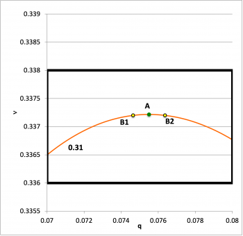
Bipolytropic (5, 1) Equilibrium Sequences 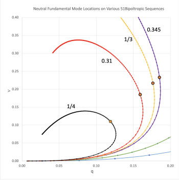
Bipolytropic (5, 1) Neutral Fundamental Mode Locations 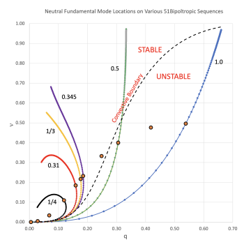
Bipolytropic (5, 1) Equilibrium Sequences
- SSC/Structure/BiPolytropes/Analytic51#Limiting_Mass


Yet Another Normalization
Fixed Core Mass
Initially, our normalization was based on holding and the central density constant. Specifically,
|
|
|
|
; |
|
|
|
|
|
|
|
; |
|
|
|
|
|
|
|
. |
|
||
We also have explored a "new normalization" based on holding and constant. Here we want to perform a Bonnor-Ebert-type analysis, examining how varies with radius if we hold and the core mass constant along an equilibrium sequence. According to our initial normalization — see, for example, here — we can write,
|
|
|
|
|
|
|
|
Therefore, from the analytic profiles that describe the core, we have,
|
|
|
|
|
|
|
|
|
|
|
|
|
|
|
|
|
|
|
|
|
|
|
|
|
|
||
|
|
||
|
|
||
|
|
||
|
|
||
|
|
||
|
|
||
|
|
||
|
|
||
|
|
||
|
|
||
|
|
||
|
|
||
|
|
Immediately below we reproduce Figure 3 from our accompanying discussion of embedded (pressure-truncated) polytropes having . Notice that frame (a) contains a plot that displays our "yet another normalization" expressions for vs. volume.
|
Equilibrium Sequences of Pressure-Truncated, n = 5 Polytropic Spheres |
|||||
| ● | †External Pressure vs. Volume (Fixed Mass) |
Mass vs. Radius (Fixed External Pressure) |
‡Mass vs. Central Density (Fixed External Pressure) |
Mass vs. Central Density (Fixed Radius) |
|
| ● | √3 | (a) |
(b) |
(c) |
(d) |
| ● | 3 | ||||
| ● | √15 | ||||
| ● | 9.01 | ||||
vs.
|
vs. |
vs. |
vs. |
||
Fixed Radius
Given that …
|
|
|
|
; |
|
|
|
|
|
|
|
; |
|
|
|
|
|
|
|
. |
|
||
we can flip from holding fixed to holding fixed via the relation,
|
|
||
|
|
||
|
|
As a result,
|
|
||
|
|
||
|
|
||
|
|
If we want to see the behavior along a sequence of the core mass, the expression is,
|
|
||
|
|
while the expression for the total mass is,
|
|
||
|
|
|
Summary: For fixed and
|
Stability
Introduction & Summary
Here we solve the LAWE numerically (on a uniformly zoned mesh — different for the separate core/envelope regions) using a 2nd-order accurate, implicit integration scheme in which the LAWE is broken into a pair of 1st-order ODEs. These results should be compared against a separate succinct discussion of our analysis obtained from integrating the LAWE in its standard 2nd-order ODE form.
| Properties of Neutral Fundamental Mode for Various Sequences | σc2 for Overtones | Ω2 for Overtones | ||||||||
 |
1st | 2nd | 1st | 2nd | ||||||
| 1.000 | 1.6639103365 | 8.4811731 | 0.49622717 | 0.53833097 | 0.000000 | 2.528013 | 5.66087 | 10.72026 | 24.0054 | |
| 0.500 | 2.2703111897 | 62.666493 | 0.399760079 | 0.305764976 | 0.000000 | 0.2659116 | 0.73022 | 8.33187 | 22.8802 | |
| 0.345 | 2.546385206 | 205.77394 | 0.232779379 | 0.185262833 | 0.000000 | 0.06741185 | 0.198075 | 6.93580 | 20.3793 | |
| 2.5675774773 | 225.75664 | 0.216806201 | 0.176420918 | 0.000000 | 0.0602615 | 0.178432 | 6.80222 | 20.1411 | ||
| 2.6095097538 | 270.59221 | 0.184909369 | 0.159274 | 0.000000 | 0.04821396 | 0.145248 | 6.52316 | 19.6515 | ||
| 2.712384289 | 415.67338 | 0.109935743 | 0.1192667 | 0.000000 | 0.02772424 | 0.088472 | 5.76211 | 18.3877 | ||
Model Sequence: μe/μc = 1.00
Marginally Unstable Model
Numbers presented in the following table should be compared against our earlier determinations. Various things to note:
- As discussed elsewhere — for example, here — when , the radial displacement function for the core — that is, for all — should be given precisely by the expression,
Hence, given that ξi = 1.6639103365 as viewed from the perspective of the core, the magnitude of, and the logarithmic derivative of the radial displacement function should have the values, respectively,
and - As discussed elsewhere — for example, here — we expect,
 NEW: |
||||||||||||||
| Mode | ||||||||||||||
| core | env | expected | measured | |||||||||||
| 1 (Fundamental) |
0.00 | 0.00 | +0.81437470 0.8154268 |
-0.455872 -0.452703 |
-1.473523 -1.471622 |
+0.3820 0.3849493 |
-1 | -0.999999992 -1.00618 |
n/a | n/a | n/a | n/a | n/a | n/a |
| 2 | 2.51513333 2.528013 |
10.7107538 10.720258 |
0.20482050 0.2069746 |
-7.09124 -7.000803 |
-5.4547441 -5.400482 |
- 0.9962 -1.018215 |
4.355376917 4.360129 |
4.35537692 4.3999485 |
0.64133 0.6456 |
0.3502 0.3444 |
n/a | n/a | n/a | n/a |
| 3 | 5.72371888 5.66087 |
24.3745901 24.0054 |
-0.14269277 -0.13587 |
+8.046019 +8.62053 |
+3.627611 +3.9723 |
+0.9308 +0.98810 |
11.18729505 11.0027 |
11.18729506 11.8164 |
0.4837 0.48395 |
0.5864 0.58326 |
0.842 0.84145 |
0.0854 0.08576 |
n/a | n/a |
| 4 | 10.3458476 | 44.0622916 | -0.20845197 | -0.6949966 | -1.61699793 | -1.1443 | 21.03114578 | 21.03114577 | 0.3939 | 0.7154 | 0.6902 | 0.2777 | 0.9115 | 0.0284 |
|
|
||||||||||||||


Model Sequence: μe/μc = 0.31
Here we examine how the frequency of the 1st overtone varies as is increased.
| Frequency Variation Along the Sequence having | ||||||||
 |
Note | 1st Overtone |  |
Fundamental | ||||
| 1.6 | 58.39858647 | 0.498473 | 14.5550593 | 0.1333725 | 3.8943827 | |||
| 2.0000 | 108.69129 | 0.236047 | 12.82812694 | 0.07011655 | 3.8105293 | |||
| 2.4000 | 199.16363 | 0.0870005 | 8.6636677 | 0.028066485 | 2.794911541 | |||
| Neutral Fundamental ==> | 2.6095097538 | 270.5922 | 0.04821396 | 6.523161 | 0.0 | 0.0 | ||
| 3.0000 | 468.1500 | 0.02329066 | 5.451761 | -0.056763527 | -13.2869232 | |||
| 3.5 | 902.640279 | 0.011747773 | 5.302006549 | - 0.098905428 | -44.63801154 | |||
| 4.0000 | 1656.926 | 0.006427613 | 5.325041 | -0.118551256677297 | -98.21535777 | |||
| 5.0000 | 4900.105 | 0.002215415 | 5.4279 | --- | --- | |||
| 6.0000 | 12544.67 | 0.000878472 | 5.510074 | --- | --- | |||
| ==> | 9.014959766 | 5.60367789 | --- | --- | ||||
| 12.0000 | 5.579608 | --- | --- | |||||
SearchMuRatio
Adding models to the above table, here we choose and iterate until we have found the value of that corresponds to the fundamental-mode. At the interface, we expect,
|
|
Throughout the core, for the neutral (i.e., ) fundamental mode of oscillation, we expect that,
|
|
Given that at the interface, we expect,
|
|
||
|
|
||
|
|
||
|
|
Similarly at the surface of the envelope for the neutral (i.e., ) fundamental mode of oscillation, we expect that,
|
|
|
||||||||||||
 |
||||||||||||
| Interface | Surface | |||||||||||
| expected |
measured | expected |
measured | |||||||||
| 1.000 | 1.6639103365 | 8.4811731 | 0.49622717 | 0.53833097 | 0.000000 | -1.471622 | -1.471622 | -1 | -1.0062 | |||
| 0.681590377 | 2.0 | 23.176456 | 0.476716895 | 0.418529653 | 0.000000 | -1.636364 | -1.636364 | -1 | -1.0078 | |||
| 0.500 | 2.2703111897 | 62.666493 | 0.399760079 | 0.305764976 | 0.000000 | -1.828212 | -1.828212 | -1 | -1.0093 | |||
| 0.425426009 | 2.4 | 108.10495 | 0.332967203 | 0.248624189 | 0.000000 | -1.948052 | -1.948052 | -1 | -1.0100 | |||
| 0.345 | 2.546385206 | 205.77394 | 0.232779379 | 0.185262833 | 0.000000 | -2.113688 | -2.113688 | -1 | -1.0108 | |||
| 2.5675774773 | 225.75664 | 0.216806201 | 0.176420918 | 0.000000 | -2.140934 | -2.140934 | -1 | -1.0110 | ||||
| 2.6095097538 | 270.59221 | 0.184909369 | 0.159274 | 0.000000 | -2.197679 | -2.197679 | -1 | -1.0112 | ||||
| 2.712384289 | 415.67338 | 0.109935743 | 0.1192667 | 0.000000 | -2.355105 | -2.355105 | -1 | -1.0117 | ||||
| 2.85 | 757.45344 | 0.034014631 | 0.068440082 | 0.000000 | -2.61723 | -2.61723 | -1 | -1.0123 | ||||
| 2.95 | 1688.1377 | 0.005065202 | 0.028486668 | 0.000000 | -2.858277 | -2.858277 | -1 | -1.0148 | ||||
| 2.995 | 8547.1981 | 0.000151797 | 0.005211544 | 0.000000 | -2.985087 | -2.985087 | -1 | -1.0132 | ||||
See Also

|
|---|
|
Appendices: | VisTrailsEquations | VisTrailsVariables | References | Ramblings | VisTrailsImages | myphys.lsu | ADS | |