SSC/Stability/BiPolytropes/51Models

BiPolytrope with n_c = 5 and n_e = 1

Here we construct and analyze the relative stability of a bipolytrope in which the core has an $n_c=5$ polytropic index and the envelope has an $n_e=1$ polytropic index.

Structure

1. Individual model profiles, taken from:
   • SSC/Structure/BiPolytropes/Analytic51#Examples
2. $(q,\nu )$ sequences of fixed ${\mu }_e/{\mu }_c$, taken from:
   • SSC/Structure/BiPolytropes/Analytic51#Model_Sequences
3. ${\nu }_{\mathrm{m}\mathrm{a}\mathrm{x}}$ model, taken from:
   • SSC/Structure/BiPolytropes/Analytic51#Limiting_Mass
      
     

     Maximum Fractional Core Mass, $\nu =M_{\mathrm{c}\mathrm{o}\mathrm{r}\mathrm{e}}/M_{\mathrm{t}\mathrm{o}\mathrm{t}}$ (solid green circular markers) for Equilibrium Sequences having Various Values of ${\mu }_e/{\mu }_c$
     $\frac{{\mu }_e}{{\mu }_c}$	${\xi }_i$	${\theta }_i$	${\eta }_i$	${\mathrm{\Lambda }}_i$	$A$	${\eta }_s$	LHS	RHS	$q\equiv \frac{r_{\mathrm{c}\mathrm{o}\mathrm{r}\mathrm{e}}}{R}$	$\nu \equiv \frac{M_{\mathrm{c}\mathrm{o}\mathrm{r}\mathrm{e}}}{M_{\mathrm{t}\mathrm{o}\mathrm{t}}}$
     $\frac{1}{3}$	$\mathrm{\infty }$	---	---	---	---	---	---	---	0.0	$\frac{2}{\pi }$
     0.33	24.00496	0.0719668	0.0710624	0.2128753	0.0726547	1.8516032	-223.8157	-223.8159	0.038378833	0.52024552
     0.316943	10.744571	0.1591479	0.1493938	0.4903393	0.1663869	2.1760793	-31.55254	-31.55254	0.068652714	0.382383875
     0.31	9.014959766	---	---	0.59835053	---	---	---	---	0.0755022550	0.3372170064
     0.3090	8.8301772	0.1924833	0.1750954	0.6130669	0.2053811	2.2958639	-18.47809	-18.47808	0.076265588	0.331475715
     $\frac{1}{4}$	4.9379256	0.3309933	0.2342522	1.4179907	0.4064595	2.761622	-2.601255	-2.601257	0.084824137	0.139370157
     Recall that, ${\ell }_i\equiv \frac{{\xi }_i}{\sqrt{3}};$       and       $m_3\equiv 3\left(\frac{{\mu }_e}{{\mu }_c}\right).$

   
    
   
   • SSC/Structure/BiPolytropes/Analytic51Renormalize#Model_Pairings
      
     

     file = Dropbox/WorkFolder/Wiki edits/Bipolytrope/Stability/qAndNuMax.xlsx --- worksheet = B-KB74 thru MinuPreparation Bipolytrope with $(n_c,n_e)=(5,1)$ Selected Pairings along the ${\mu }_e/{\mu }_c=0.31$ Sequence
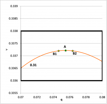
     Pairing	${\xi }_i$	${\mathrm{\Lambda }}_i$	$\nu$	$q$
     A	$9.014959766$	$0.59835053$	$0.3372170064$	$0.0755022550$
     B1	$9.12744$	$0.60069262$	$0.3372001445$	$0.0746451491$
     B2	$8.90394$	$0.59610192$	$0.33720014467$	$0.0763642133$

     
     

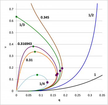
     Bipolytropic (5, 1) Equilibrium Sequences

     Bipolytropic (5, 1) Equilibrium Sequences

Stability

Here we solve the LAWE numerically (on a uniformly zoned mesh — different $\mathrm{\Delta }\tilde{r}$ for the separate core/envelope regions) using a 2^nd-order accurate, implicit integration scheme in which the LAWE is broken into a pair of 1^st-order ODEs. These results should be compared against a separate succinct discussion of our analysis obtained from integrating the LAWE in its standard 2^nd-order ODE form.

See Also