SSC/Stability/BiPolytropes/51Models

BiPolytrope with n_c = 5 and n_e = 1

Here we construct and analyze the relative stability of a bipolytrope in which the core has an $n_c=5$ polytropic index and the envelope has an $n_e=1$ polytropic index.

Structure

1. Individual model profiles, taken from:
   • SSC/Structure/BiPolytropes/Analytic51#Examples
2. $(q,\nu )$ sequences of fixed ${\mu }_e/{\mu }_c$, taken from:
   • SSC/Structure/BiPolytropes/Analytic51#Model_Sequences
3. ${\nu }_{\mathrm{m}\mathrm{a}\mathrm{x}}$ model, taken from:
   • SSC/Structure/BiPolytropes/Analytic51#Limiting_Mass
      
     

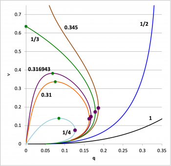
     Maximum Fractional Core Mass, $\nu =M_{\mathrm{c}\mathrm{o}\mathrm{r}\mathrm{e}}/M_{\mathrm{t}\mathrm{o}\mathrm{t}}$ (solid green circular markers) for Equilibrium Sequences having Various Values of ${\mu }_e/{\mu }_c$
     $\frac{{\mu }_e}{{\mu }_c}$	${\xi }_i$	${\theta }_i$	${\eta }_i$	${\mathrm{\Lambda }}_i$	$A$	${\eta }_s$	LHS	RHS	$q\equiv \frac{r_{\mathrm{c}\mathrm{o}\mathrm{r}\mathrm{e}}}{R}$	$\nu \equiv \frac{M_{\mathrm{c}\mathrm{o}\mathrm{r}\mathrm{e}}}{M_{\mathrm{t}\mathrm{o}\mathrm{t}}}$	$[{\xi }_i{]}_{\mathrm{s}\mathrm{m}\mathrm{o}\mathrm{o}\mathrm{t}\mathrm{h}}$
     $\frac{1}{3}$	$\mathrm{\infty }$	---	---	---	---	---	---	---	0.0	$\frac{2}{\pi }$	0.0
     0.33	24.00496	0.0719668	0.0710624	0.2128753	0.0726547	1.8516032	-223.8157	-223.8159	0.038378833	0.52024552	0.0
     0.316943	10.744571	0.1591479	0.1493938	0.4903393	0.1663869	2.1760793	-31.55254	-31.55254	0.068652714	0.382383875	0.0
     0.31	9.014959766	---	---	0.59835053	---	---	---	---	0.0755022550	0.3372170064	0.0
     0.3090	8.8301772	0.1924833	0.1750954	0.6130669	0.2053811	2.2958639	-18.47809	-18.47808	0.076265588	0.331475715	0.0
     $\frac{1}{4}$	4.9379256	0.3309933	0.2342522	1.4179907	0.4064595	2.761622	-2.601255	-2.601257	0.084824137	0.139370157	0.0
     Recall that, ${\ell }_i\equiv \frac{{\xi }_i}{\sqrt{3}};$       and       $m_3\equiv 3\left(\frac{{\mu }_e}{{\mu }_c}\right).$ Also, go here for definition of $[{\xi }_i{]}_{\mathrm{s}\mathrm{m}\mathrm{o}\mathrm{o}\mathrm{t}\mathrm{h}}$, which identifies the location of the specific-entropy step function; stability against convection is ensured whenever ${\xi }_i>[{\xi }_i{]}_{\mathrm{s}\mathrm{m}\mathrm{o}\mathrm{o}\mathrm{t}\mathrm{h}}$.

   
    
   
   • SSC/Structure/BiPolytropes/Analytic51Renormalize#Model_Pairings
      
     

     file = Dropbox/WorkFolder/Wiki edits/Bipolytrope/Stability/qAndNuMax.xlsx --- worksheet = B-KB74 thru MinuPreparation Bipolytrope with $(n_c,n_e)=(5,1)$ Selected Pairings along the ${\mu }_e/{\mu }_c=0.31$ Sequence
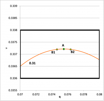
     Pairing	${\xi }_i$	${\mathrm{\Lambda }}_i$	$\nu$	$q$
     A	$9.014959766$	$0.59835053$	$0.3372170064$	$0.0755022550$
     B1	$9.12744$	$0.60069262$	$0.3372001445$	$0.0746451491$
     B2	$8.90394$	$0.59610192$	$0.33720014467$	$0.0763642133$

     
     

     Bipolytropic (5, 1) Equilibrium Sequences

     Bipolytropic (5, 1) Equilibrium Sequences

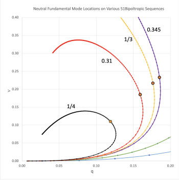
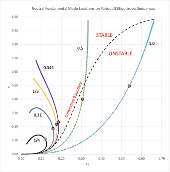
     Bipolytropic (5, 1) Neutral Fundamental Mode Locations

     Bipolytropic (5, 1) Equilibrium Sequences

Stability

Introduction & Summary

Here we solve the LAWE numerically (on a uniformly zoned mesh — different $\mathrm{\Delta }\tilde{r}$ for the separate core/envelope regions) using a 2^nd-order accurate, implicit integration scheme in which the LAWE is broken into a pair of 1^st-order ODEs. These results should be compared against a separate succinct discussion of our analysis obtained from integrating the LAWE in its standard 2^nd-order ODE form.

Properties of Neutral Fundamental Mode for Various Sequences							σc2 for Overtones		Ω2 for Overtones
	$\frac{{\mu }_e}{{\mu }_c}$	${\xi }_i$	$\frac{{\rho }_c}{\overline{\rho }}$	$\nu \equiv \frac{M_c}{M_{\mathrm{t}\mathrm{o}\mathrm{t}}}$	$q\equiv \frac{r_c}{R}$	${\sigma }_c^2$	1st	2nd	1st	2nd
	1.000	1.6639103365	8.4811731	0.49622717	0.53833097	0.000000	2.528013	5.66087	10.72026	24.0054
	0.500	2.2703111897	62.666493	0.399760079	0.305764976	0.000000	0.2659116	0.73022	8.33187	22.8802
	0.345	2.546385206	205.77394	0.232779379	0.185262833	0.000000	0.06741185	0.198075	6.93580	20.3793
	$\frac{1}{3}$	2.5675774773	225.75664	0.216806201	0.176420918	0.000000	0.0602615	0.178432	6.80222	20.1411
	$0.310$	2.6095097538	270.59221	0.184909369	0.159274	0.000000	0.04821396	0.145248	6.52316	19.6515
	$\frac{1}{4}$	2.712384289	415.67338	0.109935743	0.1192667	0.000000	0.02772424	0.088472	5.76211	18.3877

Model Sequence:  μ_e/μ_c = 1.00

Marginally Unstable Model

Numbers presented in the following table should be compared against our earlier determinations. Various things to note:

1. As discussed elsewhere — for example, here — when ${\sigma }_c^2=0$, the radial displacement function for the core — that is, for all $\xi \le {\xi }_i$ — should be given precisely by the expression,

   $x_P{|}_{n=5}$

   $=$

   $1-\frac{{\xi }^2}{15}.$

   Hence, given that ξ_i = 1.6639103365 as viewed from the perspective of the core, the magnitude of, and the logarithmic derivative of the radial displacement function should have the values, respectively,

   $x_i$

   $=$

   $0.8154268;$

   and

   $\{\frac{d\ln x}{d\ln \xi }{|}_i{\}}_{\mathrm{c}\mathrm{o}\mathrm{r}\mathrm{e}}$

   $=$

   $-\frac{2{\xi }^2}{15-{\xi }^2}=-0.45270322.$

2. As discussed elsewhere — for example, here — we expect,

   $\{\frac{d\ln x}{d\ln \tilde{r}}{|}_i{\}}_{\mathrm{e}\mathrm{n}\mathrm{v}}$	$=$	$3(\frac{{\gamma }_c}{{\gamma }_e}-1)+\frac{{\gamma }_c}{{\gamma }_e}\{\frac{d\ln x}{d\ln \xi }{|}_i{\}}_{\mathrm{c}\mathrm{o}\mathrm{r}\mathrm{e}}$
   	$=$	$3(\frac{3}{5}-1)+\frac{3}{5}\{\frac{d\ln x}{d\ln \xi }{|}_i{\}}_{\mathrm{c}\mathrm{o}\mathrm{r}\mathrm{e}}=-1.471622.$

file = Dropbox/WorkFolder/Wiki edits/BiPolytrope/TwoFirstOrderODEs/Bipolytrope51.xlsx --- worksheet = MuRatio100Fund Our September 2023 Determinations for Marginally Unstable Model Having ${\mu }_e/{\mu }_c=1$   ${\xi }_i=1.6686460157$     NEW: ${\xi }_i=1.6639103365$
Mode	${\sigma }_c^2$	${\mathrm{\Omega }}^2\equiv \frac{{\sigma }_c^2}{2}\left(\frac{{\rho }_c}{\overline{\rho }}\right)$	$x_i$	$\frac{d\ln x}{d\ln r^{*}}{|}_i$		$x_{\mathrm{s}\mathrm{u}\mathrm{r}\mathrm{f}}$	$\frac{d\ln x}{d\ln r^{*}}{|}_{\mathrm{s}\mathrm{u}\mathrm{r}\mathrm{f}}$		$\frac{r}{R}{|}_1$	$1-\frac{M_r}{M_{\mathrm{t}\mathrm{o}\mathrm{t}}}{|}_1$	$\frac{r}{R}{|}_2$	$1-\frac{M_r}{M_{\mathrm{t}\mathrm{o}\mathrm{t}}}{|}_2$	$\frac{r}{R}{|}_3$	$1-\frac{M_r}{M_{\mathrm{t}\mathrm{o}\mathrm{t}}}{|}_3$
				core	env		expected	measured
1 (Fundamental)	0.00	0.00	+0.81437470 0.8154268	-0.455872 -0.452703	-1.473523 -1.471622	+0.3820 0.3849493	-1	-0.999999992 -1.00618	n/a	n/a	n/a	n/a	n/a	n/a
2	2.51513333 2.528013	10.7107538 10.720258	0.20482050 0.2069746	-7.09124 -7.000803	-5.4547441 -5.400482	- 0.9962 -1.018215	4.355376917 4.360129	4.35537692 4.3999485	0.64133 0.6456	0.3502 0.3444	n/a	n/a	n/a	n/a
3	5.72371888 5.66087	24.3745901 24.0054	-0.14269277 -0.13587	+8.046019 +8.62053	+3.627611 +3.9723	+0.9308 +0.98810	11.18729505 11.0027	11.18729506 11.8164	0.4837 0.48395	0.5864 0.58326	0.842 0.84145	0.0854 0.08576	n/a	n/a
4	10.3458476	44.0622916	-0.20845197	-0.6949966	-1.61699793	-1.1443	21.03114578	21.03114577	0.3939	0.7154	0.6902	0.2777	0.9115	0.0284

See Also