Appendix/Ramblings/ForCohlHoward

Discussions With Howard Cohl

Motivation

These discussions began in late 2021, when Howard Cohl asked if I would be interested in working with him on establishing a better understanding of the stability of Riemann S-Type Ellipsoids. This discussion relates directly to our study of the work by 📚 N. R. Lebovitz, & A. Lifschitz (1996, ApJ, Vol. 458, pp. 699 - 713).

We are motivated to pursue this discussion, in part, because our own research group at LSU has previously carried out some nonlinear dynamical simulations that relate to this topic. See …

• YouTube Simulation that draws from the following ApJ publication.
• Relevant Publication:   📚 S. Ou, J. E. Tohline, & P. M. Motl (2007, ApJ, Vol. 665, pp. 1074 - 1083), titled, Further Evidence for an Elliptical Instability in Rotating Fluid Bars and Ellipsoidal Stars.

  Publication Abstract Using a three-dimensional nonlinear hydrodynamic code, we examine the dynamical stability of more than 20 self-gravitating, compressible, ellipsoidal fluid configurations that initially have the same velocity structure as Riemann S-type ellipsoids. Our focus is on adjoint configurations, in which internal fluid motions dominate over the collective spin of the ellipsoidal figure; Dedekind-like configurations are among this group. We find that, although some models are stable and some are moderately unstable, the majority are violently unstable toward the development of m=1, m=3, and higher-order azimuthal distortions that destroy the coherent, m=2 barlike structure of the initial ellipsoidal configuration on a dynamical timescale. The parameter regime over which our models are found to be unstable generally corresponds with the regime over which incompressible Riemann S-type ellipsoids have been found to be susceptible to an elliptical strain instability. We therefore suspect that an elliptical instability is responsible for the destruction of our compressible analogs of Riemann ellipsoids. The existence of the elliptical instability raises concerns regarding the final fate of neutron stars that encounter the secular bar-mode instability and regarding the spectrum of gravitational waves that will be radiated from such systems.

  Initial frame of a YouTube animation that shows one model's evolution

Understanding the Dimensionality of EFE Index Symbols

Howard put together a Mathematica script intended to provide — for any specification of the semi-axis length triplet $(a,b,c)$ — very high-precision, numerical evaluations of any of the index symbols, $A_{ijk\dots }$ and $B_{ijk\dots }$ as defined by Eqs. (103 - 104) in §21 of [EFE]. Originally I suggested that, without loss of generality, he should only need to specify the pair of length ratios, $(1,b/a,c/a)$. In response, Howard pointed out that evaluation of all but a few of the lowest-numbered index symbols — as defined by [EFE] — does explicitly depend on specification of (various powers of) the semi-axis length, $a$.

Joel's response:  Howard is correct! He should leave the explicit dependence of $a$ — to various powers — in his Mathematica notebook's determination of all the EFE index symbols.

Instead, what we should expect is that the evaluation of various physically relevant parameters will produce results that are independent of the semi-axis length, $a$; these evaluations should involve combining various index symbols in such a way that the dependence on $a$ disappears. Consider, for example, our accompanying discussion (click to see relevant expressions) of the virial-equilibrium-based determination of the frequency ratio, $f\equiv \zeta /{\mathrm{\Omega }}_f$, in equilibrium S-Type Riemann Ellipsoids. Although most of the required index symbols, $A_1,A_2,A_3$ and $B_{12}$, are dimensionless parameters, the index symbol $A_{12}$ has the unit of inverse-length-squared. Notice, however, that when $A_{12}$ appears along with any of these other dimensionless parameters in the definition of $f$, it is accompanied by an extra "length-squared" factor, such as $a^2$. Hence, although I strongly agree that Howard should continue to include various powers of $a$ (etc.) in his Mathematica notebook expressions, I suspect that, without loss of generality, in the end we will always be able to set $a=1$ and only need to specify the pair of length ratios, $(1,b/a,c/a)$.

Evaluation of Index Symbols

Three Lowest-Order Expressions

In our accompanying derivation of expressions for the three lowest-order index symbols $A_i$, we have used subscripts $(\ell ,m,s)$ instead of $(1,2,3)$ in order to identify which associated semi-axis length is (largest, medium-length, smallest). We have derived the following expressions:

$\frac{A_{\ell }}{a_{\ell }{a}_m{a}_s}$ $=$ $\frac{2}{a_{\ell }^3{p}^2{\sin }^3\alpha }[F(\alpha ,p)-E(\alpha ,p)];$ $\frac{A_m}{a_{\ell }{a}_m{a}_s}$ $=$ $\frac{2}{a_{\ell }^3}\left[\frac{E(\alpha ,p)-(1-p^2)F(\alpha ,p)-(a_s/a_m)p^2\sin \alpha }{p^2(1-p^2){\sin }^3\alpha }\right];$ $\frac{A_s}{a_{\ell }{a}_m{a}_s}$ $=$ $\frac{2}{a_{\ell }^3}\left[\frac{(a_m/a_s)\sin \alpha -E(\alpha ,p)}{(1-p^2){\sin }^3\alpha }\right].$

The corresponding expressions that appear in Howard's Mathematica notebook are:

$A_1$ $=$ $\frac{2a_2{a}_3}{a_1^{2}m{\sin }^3(\varphi )}[\mathrm{E}\mathrm{l}\mathrm{l}\mathrm{i}\mathrm{p}\mathrm{t}\mathrm{i}\mathrm{c}\mathrm{F}[\varphi ,m]-\mathrm{E}\mathrm{l}\mathrm{l}\mathrm{i}\mathrm{p}\mathrm{t}\mathrm{i}\mathrm{c}\mathrm{E}[\varphi ,m]];$ $A_2$ $=$ $\frac{2a_2{a}_3}{a_1^{2}m(1-m){\sin }^3(\varphi )}[\mathrm{E}\mathrm{l}\mathrm{l}\mathrm{i}\mathrm{p}\mathrm{t}\mathrm{i}\mathrm{c}\mathrm{E}[\varphi ,m]-{\cos }^2\theta \cdot \mathrm{E}\mathrm{l}\mathrm{l}\mathrm{i}\mathrm{p}\mathrm{t}\mathrm{i}\mathrm{c}\mathrm{F}[\varphi ,m]-\frac{a_3}{a_2}\cdot {\sin }^2\theta \sin \varphi ];$ $A_3$ $=$ $\frac{2a_2{a}_3}{a_1^2(1-m){\sin }^3(\varphi )}[\frac{a_2}{a_3}\cdot \sin (\varphi )-\mathrm{E}\mathrm{l}\mathrm{l}\mathrm{i}\mathrm{p}\mathrm{t}\mathrm{i}\mathrm{c}\mathrm{E}[\varphi ,m]].$

With a little study it should be clear that our derived expressions for $A_i$ precisely match Howard's Mathematica-notebook expressions when $\ell =1$, $m=2$, and $s=3$, that is, in all cases for which $a_1>a_2>a_3$. But there will be models to consider (for example, in the uppermost region of the so-called "horn-shaped" region for S-Type Riemann Ellipsoids) for which $a_1>a_3>a_2$, in which case care must be taken in assigning the proper expressions to $A_2$ and $A_3$. Similarly note that most of the Riemann models of Type I, II, and III — see, for example, Figure 16 (p. 161) in Chapter 7 of [EFE] — have either $a_2>a_1$ or $a_3>a_1$.

Determination of Higher-Order Expressions

Howard's Mathematica notebook performs brute-force integrations to evaluate various higher-order index-symbol expressions. Why doesn't he instead use recurrence relations, which point back to the elliptic-integral-based expressions for $A_1,A_2,A_3$? Specifically …

Index-Symbol Recurrence Relations
$B_{ijk\ell \dots }$	$=$	$A_{jkl\dots }-a_i^2{A}_{ijkl\dots }$
[EFE], §21, p. 54, Eq. (105)
$a_i^2{A}_{ikl\dots }-a_j^2{A}_{jkl\dots }$	$=$	$+(a_i^2-a_j^2)B_{ijk\ell \dots }$
[EFE], §21, p. 54, Eq. (106)
$A_{ikl\dots }-A_{jkl\dots }$	$=$	$-(a_i^2-a_j^2)A_{ijk\ell \dots }$
[EFE], §21, p. 54, Eq. (107)

For example, setting $i=1$ and $j=2$ in the third of these expressions gives,

$A_1-A_2$	$=$	$-(a_1^2-a_2^2)A_{12}$
$\Rightarrow A_{12}$	$=$	$\frac{A_2-A_1}{(a_1^2-a_2^2)}$
$\Rightarrow a_1^2{A}_{12}$	$=$	$\frac{A_2-A_1}{(1-a_2^2/a_1^2)};$

and, from the first of the relations,

$B_{12}$	$=$	$A_2-a_1^2{A}_{12}$
	$=$	$A_2-a_1^2\left[\frac{A_2-A_1}{(a_1^2-a_2^2)}\right]$
	$=$	$\frac{1}{(a_1^2-a_2^2)}[(a_1^2-a_2^2)A_2-a_1^2(A_2-A_1)]$
	$=$	$\frac{1}{(a_1^2-a_2^2)}[a_1^2{A}_1-a_2^2{A}_2]$
	$=$	$\frac{1}{(1-a_2^2/a_1^2)}[A_1-\frac{a_2^2}{a_1^2}\cdot A_2].$

Also, consider using the set of relations labeled "LEMMA 7" on p. 54 of [EFE].

Example Test Evaluations

Some of Howard's 20-digit-precision evaluations of various index symbols have been recorded, for comparison with our separate lower-precision evaluations, as follows:

• Values of $(A_1,A_2,A_3)$ are recorded for a model with $(a_1,a_2,a_3)=(1,0.9,0.641)$ in the table titled, TEST (part 1), near the top of our chapter on Riemann S-Type ellipsoids.
• Values of $(A_{12},B_{12})$ are recorded for a model with $(a_1,a_2,a_3)=(1,0.9,0.641)$ in the table titled, TEST (part 2) in our chapter on Riemann S-Type ellipsoids.

Figures circa Year 2000

Approximately four years after 📚 Lebovitz & Lifschitz (1996) was published, Norman Lebovitz gave a copy of his stability-analysis (FORTRAN) code to Howard Cohl. Using this code, Howard was able to generate a large set of growth-rate data that essentially allowed him to reproduce Figure 2b from 📚 Lebovitz & Lifschitz (1996).

Image i3.png

Howard's plot of this data — his image i3.png — is shown immediately below; the abscissa is $0\le b/a\le 1$ and the ordinate is $0\le c/a\le 1$.

Howard's "i3.png" image
Compare with Figure 2b of 📚 N. R. Lebovitz, & A. Lifschitz (1996, ApJ, Vol. 458, pp. 699 - 713)

Image i5.png

In an effort to better examine growth-rate trends in the lower-left quadrant of this 📚 Lebovitz & Lifschitz (1996) figure, Howard plotted the same set of stability-analysis data on an axis pair where the abscissa is still $0\le b/a\le 1$, but where, for each value of $b/a$, the ordinate extends from the lower self-adjoint sequence to the upper self-adjoint sequence — labeled, respectively, $x=+1$ and $x=-1$ in the classic EFE diagram (EFE, §49, p. 147, Fig. 15 or, see our accompanying discussion). This is displayed immediately below as Howard's "i5.png" image.

Howard's "i5.png" image
Notice …

In generating his "i5.png" image, precisely how did Howard "stretch" the ordinate from $c/a$ (as used in his "i3.png" image) to an ordinate ranging from the lower to the upper self-adjoint sequences? Drawing from 📚 Lebovitz & Lifschitz (1996) I presume that, for a given point in the EFE diagram $(b/a,c/a)$, Howard used the expression,

$x_{\pm }$	$=$	$-C\pm \sqrt{C^2-1},$
📚 Lebovitz & Lifschitz (1996), §2, p. 701, Eq. (8)

where,

$C$	$\equiv$	$\frac{ab{B}_{12}}{c^2{A}_3-b^2{a}^2{A}_{12}},$
📚 Lebovitz & Lifschitz (1996), §2, p. 701, Eq. (6)

Then I presume that the ordinate, $y$ — which runs from zero to unity in the "i5.png" image — is determined from the expression,

$y$

$=$

$0.5(1-x_{\pm }).$

Is this the way Howard generated "i5.png"?

In an email dated 26 January 2022, Howard provided the following answer to this question — I had numerical data that I think Norman provided me for the lower and upper self-adjoint sequences. They were simply two sets of curvilinear data in the (b/a,c/a) diagram. Call ay=b/a and then az=c/a. Then lsa and usa are both functions of ay. Note that when I encountered points which didn't lie on Norman's data, I interpolated using a 9th degree polynomial to the lower and upper self-adjoint sequence data. Now consider that you have some data "g" which gives you points in the (ay,az) plane, then g=g(ay,az). Take for instance data "g" which are points in the (ay,az) plane where the growth rate are above some critical value such as 10e-5. For every data point g, there is a fixed ay coordinate value. Normally you would plot that point at (ay,az). The remapping that I did now plots it instead at a point on the ordinate given by some az'= (az-lsa(ay))/(usa(ay)-lsa(ay)) So if az=lsa(ay) then it appears at the ordinate value of zero. and if az=usa(ay) then it appears at the ordinate value of unity. So the whole horn shaped region is mapped into the unit square.

Image i4.png

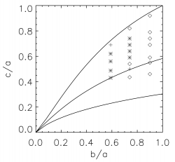
Howard's "i4.png" image, immediately below, presents a magnification of the upper-right-hand portion (identified, by hand, as the "E-group") of his "i5.png" image. The abscissa spans the parameter range, $0.3\le b/a\le 1.0$ while the ordinate spans the parameter range, $0.96\le y\le 1$.

Howard's "i4.png" image
Notice …

Summary

Howard is interested in understanding — in greater detail than appears in 📚 Lebovitz & Lifschitz (1996) — what gives rise to, and what is the extent of these various bands of instability in the classic EFE diagram. Explicit comments/questions:

1. Notice in "i4.png" that the bands labeled E4, E6, and E8 appear to extend all the way to, and intersect, the Maclaurin spheroid sequence.

Self-Adjoint Sequences

In an email dated 26 January 2022, Howard asked, "Do you have analytic curves for the lower and upper self-adjoint sequences? Otherwise, do you have very accurate data for the lower and upper self-adjoint sequences?"

On the same day, I sent the following response to Howard:

I have added a subsection to my online chapter discussion of 📚 Lebovitz & Lifschitz (1996) in which I derive an expression whose solution/root should map out the **upper** boundary (x = -1) of the horned-shape region. Click here to see the entire derivation; this derivation ends with the following recommended strategy:

STRATEGY for finding the locus of points that define the upper boundary of the horned-shape region …    Set $a=1$, and pick a value for $0<b<1$; then, using an iterative technique, vary $c$ until the following expression is satisfied: $[c^2(a+b)+a{b}^2]\left[\frac{(b/a)\sin \theta -(c/a)E(\theta ,k)}{(1-k^2){\sin }^3\theta }\right]$ $=$ $a^{2}b+bc(a-b)\left[\frac{F(\theta ,k)-E(\theta ,k)}{k^2{\sin }^3\theta }\right].$ Choose another value of $0<b<1$, then iterate again to find the value of $c$ that corresponds to this new, chosen value of $b$. Repeat!

Related remarks:

1. I have not actually plugged in numbers -- that is, (b,c) pairs -- to see if it works, but I am pretty confident in the result because the derivation was pretty straightforward. Would you mind trying it out for me, since you have working elliptic integral routines?
2. It would be wise to start by trying to duplicate -- then improve upon -- the set of (b, c) coordinate-pairs that were derived by Chandrasekhar and presented in EFE Table VI (section 48, p. 142).
3. Shortly, I will derive the complementary expression that maps out the "lower" boundary (x = +1).

On 27 January 2022, Joel added a subsection to the online chapter discussion of 📚 Lebovitz & Lifschitz (1996) in which he derives an expression whose solution/root should map out the **lower** boundary (x = +1) of the horned-shape region. Click here to see the entire derivation; this derivation ends with the following recommended strategy:

STRATEGY for finding the locus of points that define the lower boundary of the horned-shape region …    Set $a=1$, and pick a value for $0<b<1$; then, using an iterative technique, vary $c$ until the following expression is satisfied: $[c^2(a-b)+a{b}^2]\left[\frac{(b/a)\sin \theta -(c/a)E(\theta ,k)}{(1-k^2){\sin }^3\theta }\right]$ $=$ $a^{2}b-bc(b+a)\left[\frac{F(\theta ,k)-E(\theta ,k)}{k^2{\sin }^3\theta }\right].$ Choose another value of $0<b<1$, then iterate again to find the value of $c$ that corresponds to this new, chosen value of $b$. Repeat!

 

Upper (USA) and Lower (LSA) Self-Adjoint (Howard's Compact Expressions Plus Plot 1/28/2022) (tabulated data here)

COLLADA 3D Animations

DOWNLOADABLE 3D MODELS

Riemann Type I Ellipsoids

Click here.

Excerpts From Various Lebovitz Publications Regarding Stability Studies

"… the onset of instability is not very sensitive to the compressibility or angular momentum distribution of the polytrope when the models are parameterized by T/|W| — [in particular, the m = 2 barmode becomes unstable at T/|W| ∼ 0.26 - 0.28. ] The polytrope eigenfunctions are … qualitatively different from the Maclaurin eigenfunctions in one respect: they develop strong spiral arms. The spiral arms are stronger for more compressible polytropes and for polytropes whose angular momentum distributions deviate significantly from those of the Maclaurin spheroids."

— Drawn from Toman, Imamura, Pickett & Durisen (1998), ApJ, 497, 370

See Also

• MediaWiki chapter on Riemann S-Type Ellipsoids     <==     includes Self-Adjoint Data Table from EFE and from Howard's high-precision (20-digit accuracy) evaluation.
• MediaWiki chapter on Lebovitz & Lifschitz (1996)    <==     Analytic expressions that give the location of the Self-Adjoint Sequences in the EFE Diagram is presented here.
• 📚 S. Ou, J. E. Tohline, & P. M. Motl (2007, ApJ, Vol. 665, pp. 1074 - 1083), titled, Further Evidence for an Elliptical Instability in Rotating Fluid Bars and Ellipsoidal Stars.